Bifurcation Analysis of One-Dimensional Dynamical Systems
Last time we learned how to compute fixpoints and their stability of one-dimensional dynamical systems to investigate their asymptotic behavior.
Now let's look at this in more detail. The examples in the lecture and discussed in the notes were all systems that had parameters. Recall the SIS system
[ \dot x=\alpha\left(x(1-x)-\frac{1}{R_{0}}x\right) ]
that exhibited different types of asymptotic behavior depending on the value of the basic reproduction number $R_0$.
Let's take this perspective now. Instead of asking how does $x(t)$ depend on time we ask:
How does the asymptotic behavior depend on the parameters?
Let's assume we have a dynamical system
[ \dot{x}=f(x;\mu) ] that only depends on one parameter $\mu$. Since one-dimensional dynamical systems are determined by the set of fixpoints, we can use them to see how the behavior changes as $\mu$ is varied (i.e. how the set of fixpoints and their stability changes). Consider the example in the panel below.
**Panel 1: Preliminary Bifurcation Analysis** of the function $f(x)=\sin(3 x) + x\^2/5 +\mu $. By varying the parameter $\mu$ the set of fixpoints changes, pairs of stable and unstable fixpoints are created or annihilated by "collision". With the slider you can change the control parameter $\mu$, effectively shifting the function up and down.
This is the dynamical system [ \dot{x}=f(x)=\sin(3x)+x^{2}/5+\mu. ] As we vary the parameter $\mu$ we see that a sequence of events happens to the set of fixpoint. As we decrease the parameter $f(x)$ crosses the $x-$axis and pairs of stable and unstable fixpoints are created or merge and annihilate. These events are called bifurcations. In the above example, they are all defined by the creation or annihilation of fixpoints of different types. Because quite often even a complex function $f(x)$ is just a curve with minima and maxima and if the control parameter $\mu$ is just a constant added to $f(x)$ it pushes the function up and down and generically maxima and minima cross the $x$-axis yielding these bifurcations. They are called saddle-node bifurcations for reasons that will become clear later.
Saddle node bifurcations
Let's study this in a simple model that has exactly one such saddle node bifurcation: [ \dot{x}=f(x)=x^{2}+\mu ] If we plot $f(x)$ for different values of $\mu$ we see that three different scenarios emerge (Panel 2):
**Panel 2: Saddle node bifurcation**
When $\mu<0$ two fixpoints exist, one is stable one is not. The fixpoints are [ x^{\star}=\pm\sqrt{\mu} ] As $\mu$ is increased these fixpoints approach each other and when $\mu=\mu_{c}=0$ the system has one fixpoint that attracts everything from the left but repels everything on the right. It's marginally stable. When $\mu$ is increased further, the fixpoint disappears. In a sense, the stable and unstable fixpoints annihilate by "collision".
Now instead of drawing $f(x)$ for different values of $\mu$ we can draw a Bifucation diagram. This is a plot, that depicts the stationary states (on the y-axis) vs. the control parameter $\mu$ (on the x-axis). Why? Because we are really interested in treating the control parameter as an independent control variable and the asymptotic behavior as the dependent variable. This is then what we get:
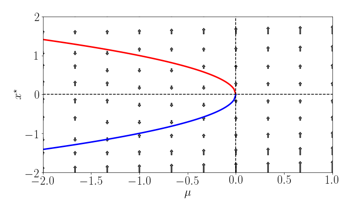
**Figure 1: Saddle node bifurcation diagram**: The control parameter is on the "x"-axis and the stationary states on the "y"-axis. The fixpoints are shown as a function of the control parameter $\mu$. Red means unstable, blue stable. The dynamics, the flow of trajectories is indicated by arrows.
This is a bifurcation diagram it illustrates the asymptotic behavior of a dynamical system as a function of its parameter.
Bifurcartion diagrams show comprehensively how a dynamical systems behaves for all possible parameter choices. It therefore provides a global view of the system.
This is often very important because in many applications we would like to know what potential behaviors a system can exhibit, not necessarily what behavior it exhibits at a given parameter choice.
Transcritical bifurcation
**Panel 3: Transcritical Bifurcation:** Two fixpoints exchange stability.
In turns out that in addition to the saddle node bifurcation we can have other types of bifurcations. For example the transcritical bifurcation (Panel 3).
This is when a stable and unstable fixpoint collide and interchange their stability properties. Here's the generic example:
[ \dot{x}=f(x;\mu)=\mu x-x^{2}=x(\mu-x). ] This guy always has a fixpoint at $x=0$ and one at $x=\mu$. However, for $\mu<0$ this second fixpoint is on the left of the origin and for $\mu>0$ it's on the right, see Panel 3.
If we look at the bifurcation diagram, we see that the fixpoints collide and exchange their stability properties:
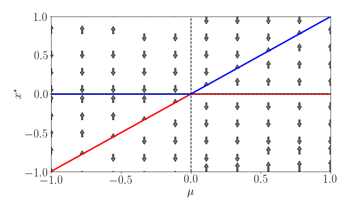
**Figure 2: Transcritical Bifurcation:** the two fixpoints at $x\^\star=0$ and $x\^\star=\mu$ exchange their stability at the critical control parameter value $\mu=0$.
Pitchfork bifurcation
**Panel 4: The pitchfork bifurcation:** A fixpoint has two babies that inherit mom's stability, while mom changes her stability.
There's another type of bifurcation frequently encountered. Let's look at [ \dot{x}=f(x;\mu)=\mu x-x^{3}=x(\mu-x^{2}). ] Here we also have always a fixpoint $x^{\star}=0$. However, for $\mu>0$ we have two additional fixpoints [ x^{\star}=\pm\sqrt{\mu}. ] You can check for yourself in Panel 4.
What happens here is this: Let's start with $\mu<0$. The system has a single stable fixpoint at the origin. As we increase $\mu$ this stable fixpoint gives birth to two new stable fixpoints at $\mu=\mu_{c}=0$ and loses its own stability. The bifurcation diagram looks like a pitchfork which is why this type of bifurcation is called pitchfork bifurcation.
This is what the bifurcation diagram looks like:
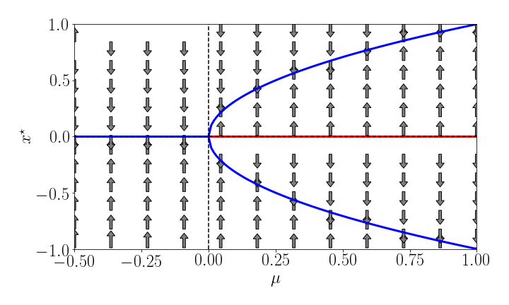
**Figure 3: The Pitchfork Bifurcation:** The bifurcation diagram looks like a pitchfork.
It can also happen that an unstable fixpoint gives birth to two new unstable fixpoints and becomes a stable fixed point.
Saddle node, transcritical and pitchfork bifurcations are the most important bifurcations in 1d systems. There are more types of bifurcation but they are not as common.
Application: Cell differentiation
The pitchfork bifurcation has some interesting properties that we can use to think about systems that possess a single stable attractor and undergo a slow parameter change and when a critical parameter value is crossed the original stable state becomes unstable and two competing, new stable attractors emerge.
For example we can think of the original singular stable state as a stem cell and a slow parameter change as some changes in the environment that push the system into a parameter regime in which two stable states emerge that reflect different differentiation states that a stem cell can develop into.
So as a qualitative model we could say that the system is governed by the dynamical system
[ \dot{x}=f(x;\mu)=x(\mu-x^{2}). ]
in which $x(t)$ represents the state of a cell and we imagine that the parameter $\mu$ is controlled by some environmental factors.
In addition we say that the state is not fully governed by the above ODE but we also have some noise that can change the state
[ \dot{x}=f(x;\mu)=x(\mu-x^{2})+\text{Noise}. ]
There's a way to model this noise and we can be more specific about it. It's a topic that we will cover later. For now imagine that the noise will add little random changes to the state so that instead of moving along smooth curve there's a bit of a wiggle force acting on the state variable. What we have in mind here becomes clearer if we look at the difference equation again: [ x(t+\Delta t)\approx x(t)+\Delta tf(x(t))+\Delta W(t) ] at every point in time we add a random number $\Delta W(t)$ that is drawn from a normal distribution with a small variance and zero mean. If this is too vague at the moment, don't worry. We will be more specific when we cover stochastic differential equations. Right now, let's just think that as time goes one there's always a little random change in $x(t)$.
Let's now investigate what happens in the above system if we start with a control parameter $\mu<0$ and slowly increasing $\mu$. You can try this with the slider in Panel 5.
**Panel 5: Dynamics of a system with a pitchfork bifurcation**: The dot is the state of the system. The wiggling reflects that in addition to the deterministic ODE part of the dynamical system, the state is subject to a bit of noise. As you slowly increase the control parameter, the state will make a choice on which branch of the pitchfork to go.
We see that in the initial regime the state wiggles around its only stable solution. As we slowly increase the control parameter, even into the region $\mu>0$ the state will remain there for a bit and then either approach the top branch or the bottom branch, so with a 50/50 chance one of the stable attractors. In our analogy of cell differentiation the cell fate is going to one of two possible states.
If we decrease the control parameter again, we will see that the system goes back to the original state.
Hysteresis
So far, when we changed the control parameter of a system in some equilibrium state $x^{\star}$ the value of this equilibirum changes slowly, even as we pass a critical point. The above example showed that we can go from a regime with one equilibrium to one with two of them and back. But as we change the control parameter the asymptotic state changes continuously from the stable state onto one of the other stable branches and back.
However, the existence and interplay between bifurcations can yield some interesting behavior when many bifurcations exist. Let's look at the following example. Let's say that we have a dynamical system defined by [ \dot{x}=-x(x-1)(x+1)+\mu+\text{Noise}. ] Just like above, we imaging that the system is also under the influence of noise which makes it wiggle around its stable asymptotic state.
The bifurcation diagram of this system is depicted in Panel 6.
**Panel 4: Hysteresis:** Here's a system that has two saddle node bifurcartions at two different critical parameter values $\mu=\pm 2/3\sqrt(3)$. in the intermediate range the system has three fixpoints, the middle one is undstable. When the system is initially at a control parameter less that the left critical value, the state remains in its only stable fixpoint. As the parameter is increased, the saddle-node bifurcation creates two additional fixpoints but the state doesn't "sense" them. When the second critical point is reached the stable branch on the bottom disappears by a collision of two fixpoints. At that state the state undergoes a massive change and jumps to the upper branch. Decreasing the control parameter will not result in a return to the lower stable branch, the system will remain in the upper branch.
The key behavior here is that as the control parameter is changed slowly the system will remain on the stable branch and will not "sense" the emergence of an alternative stable state. However when the bottom stable branch gets annihilated the state has no choice but to jump to the upper branch. This implies a small parameter change can have a massive effect on the state. Also, if one decides to decrease $\mu$ again, the state will not return to the original lower branch, but rather stick to the upper branch until that one disappears when $\mu$ gets too small.
This behavior is known as hysteresis and can play a role in a number of dynamical systems. Because only saddle-node bifurcations are involved, we can expect this behavior to occur generically in many systems that exhibit multi-stability.