One Dimensional Dynamical Systems
Last time we discussed one-dimensional discrete-time maps [ x_{n+1}=f(x_{n}) ]
with initial condition $x_{0}$ and evolving in discrete steps $n=0,1,2,...$ . We discovered that, for example, in spite of its simplicity the logistic map
[ x_{n+1}=\lambda x_{n}(1-x_{n}) ]
exhibits some interesting and unexpected behavior like deterministic chaos and self-similarity in the bifurcation diagram. One of the key features of discrete maps is that they possess no restrictions on the magnitude of change going from state $x_{n}$ to state $x_{n+1}$. For example, no assumptions are made that the difference $\Delta x_{n}=x_{n+1}-x_{n}$ is small compared to $x_{n}$. Also there's no talk about what a time step means in terms of physical time or time units. In a number of dynamical systems across all fields we do have some information about this. We observe systems that change a bit in small time intervals and need more time to change significantly. In fact, there are lots of systems like this which actually give us the notion of time and time-scale.
Small times and small changes
In many systems the properties of the system are such that we can work with the assumption that for small times changes in the system are also small. This implies that we need to work with a time-axis that is suitable for saying: ``this is a small time interval''.
Typically this is best discussed in systems in which we view time $t$ as a continuous variable and refer to $x(t)$ as the state of the system at time $t$. In some of the applications that we will discuss $x(t)$ could be the concentration of an intracellular chemical compound or some substance, or the fraction of individuals in a population of a particular type, for example infected individuals in a population that is exposed to an epidemic, or particles in a reaction. In many applications, we have situations in which the state variable is derived from a quantity that is discrete, that we can count, like the number of people, but the number is typically large so we can think of it as a continuous quantity, or we can think of it as an expected number (which doesn't have to be discrete). We will discuss this in more detail later. For now let's assume that we have a continuous quantity that describes the state of the system and we denote it by $x(t)$.
**Panel 1: A particle annihilation system.** Initially we have $x(t_0)$ particles in a box. When they collide they annihilate. What is the expected $x(t)$?
Example: Particles in a box that annihilate on collision
Let's use a simple example to explain. Let's assume that we have a container of molecules of type $A$ and when two molecules collide they annihilate and disappear like so: [ A+A\xrightarrow{\alpha}\emptyset ]
Let's assume that initially ($t=t_{0}$) we have some amount of molecules in the container which we denote by $x(t_{0})$ measured for example in mol. We have a system in mind in which the container is well mixed so each given pair of molecules has a fixed probability of interacting.
Just by looking at the reaction above we see already that $x(t)$ must be decreasing because particles only get destroyed. But if we want to understand a bit more about the system for instance in what way $x(t)$ may decrease over time. Will it decrease exponentially? Algebraically? If so what is the exponent?
In Panel 1 you can experiment a bit with the system.
We can develop a model based on a few plausible assumptions. Let's assume that we know $x(t)$ and look at the system a small time $\Delta t$ later. We choose this time as small as we like thinking that the smaller it gets, the smaller the expected change in $x(t)$. If we assume this we can write [ x(t+\Delta t)\approx x(t)+\Delta t\,f(x(t)) ]
so the state of the system shortly after our reference time $t$ is the old state plus a change that is proportional to $\Delta t$. The proportionality constant is $f(x(t))$ which may depend on the state we are in. This then naturally yields [ \lim_{\Delta t\rightarrow0}\frac{x(t+\Delta t)-x(t)}{\Delta t}=\frac{dx}{dt}=f(x) ]
which we write has [ \dot{x}=f(x) ]
So the rate at which our state variable changes is given by the function $f(x)$. So we have, based on our assumptions, a system that can be described by an ordinary differential equation (ODE) in one dimension. Typically, in modeling projects ODEs are written down from the very start and it appears that modelers sometimes forget about the assumptions that have been made in order for these types models to be valid. Always remember what assumptions ODE models are based on.
For the above particle annihilation example we can now try to derive the appropriate $f(x)$. Remember that $x(t)$ is the number or abundance particles.
Now let's assume the perspective of a single $A$ molecule labeled $i$. In the time interval $t,t+\Delta t$ this single molecule can encounter another particle $j$ and both can annihilate. The probability that our marked molecule encounters any other particle should be proportional to the abundance of the molecules altogether. So the expected change in the abundance caused by a single molecule $i$ is
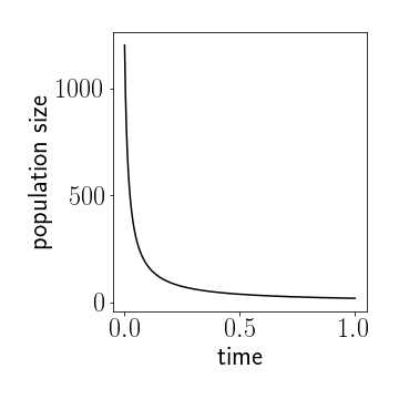
**Figure 1:** The solution $x(t)$ to the ODE model for a population of particles that annihilate. Here we $x(0)=1200$ and $\alpha=0.01$.
[ \Delta x_{i}=-\alpha x(t)\Delta t ]
where $\alpha$ is a proportionality constant and the subscript $i$ indicates that this is the expected change in $x(t)$ caused by particle $i$. Because every particle, not only $i$, can contribute to the change, the total change in the small time-interval is [ \Delta x=\sum_{i}\Delta x_{i}=-\alpha x(t)x(t)\Delta t ]
which yields the ODE: [ \dot{x}=-\alpha x^{2}. ]
We can solve this directly by separation of variables [ -\frac{dx}{\alpha x^{2}}=dt ]
and integrating [ \frac{1}{\alpha x(t)}-\frac{1}{\alpha x(t_{0})}=t-t_{0} ]
so [ x(t)=\frac{x(t_{0})}{1+\alpha x(t_{0})(t-t_{0})} ] For $t>t_{0}$. So, as $t$ becomes very large the abundance decreases as $\sim1/t$ and approaches zero, as expected. The good thing is, we now know that the decreases is as $1/t$, see Figure 1.
Let's make this a bit more interesting....
....and look at two different reactions, the annihilation reaction [ A+A\rightarrow\emptyset ] and the spontaneous reproduction reaction [ A\rightarrow2A. ] We can see already that the second reaction can generate new molecules. Alternatively, we can think of organisms here. Individuals can reproduce (as in the logistic map) driven by the second equation and kill each other which is captured by the first equation. Below is a simulation of this system.
**Panel 2: Reproduction and annihilation.** Here's a system of particles in a box. Inititally, we have a few particles at low concentration. These particles can replicate at a ***reproduction rate***. When they collide they annihilate. You can vary the these parameters with the sliders. ***Start by pressing play*** and wait a bit until the particle number increases. When the density is sufficiently high, particles will start to annihilate. Eventually an equilibrium is reached.
Now the change of the abundance caused by the second equation is always positive, each $A$ can spontaneously spawn a new $A$, so the change in $x(t)$ is proportional to $x(t)$ and positive [ \Delta x=\beta x \Delta t ] where $\beta$ is a proportionality constant. In combination with the annihilation reaction this yields the system [ \dot{x}=\beta x-\alpha x^{2} ] which we write as [ \dot{x}=x(\beta-\alpha x) ] Now let's recall what we are modeling here. $x(t)$ is an abundance or concentration so it cannot be negative, i.e. $x(t)\geq0$. The parameters $\alpha$ and $\beta$ are positive. Now we could go ahead and solve this ODE by separation of variables and integrating the equation [ \int_{x(t_{0})}^{x(t)}\frac{dx}{x(\beta-\alpha x)}=\int_{t_{0}}^{t}dt ] which is
- possible but
- neither fun
- nor necessary
This is why: Let's look at the dynamical system again: [ \dot{x}=x(\beta-\alpha x). ]
In what follows we set the beginning of time $t_{0}=0$ and have $x(0)=x_{0}\geq0$ as the initial condition. If $x_{0}=0$ then $\dot{x}=0$ which implies that there is no change in $x(t)$. If $x(0)=0$ then $x(t)=0$ for all times. Likewise, if $x_{0}=\beta/\alpha$ we have $\dot{x}=0$ and $x(t)=\beta/\alpha$ for all times.
Fixpoints and their stability
These points are stationary points or fixpoints analogous to the discrete map discussed last time. Here however the condition for a fixpoint is [ \dot{x}=f(x)=0 ] whereas in the discrete map it is [ x_{n+1}=x_{n}=f(x_{n}) ] which is very different and a consequence of the fact that the ODE systems are designed to model systems that have a particular behavior for small times, namely that changes also become small as $\Delta t$ becomes small.
Now, the ODE system above has two fixpoints [ x_{1}^{\star}=0 ] and [ x_{2}^{\star}=\beta/\alpha>0 ] If we start at any value except these two points we will find that every initial condition yields a trajectory [ x(t)\rightarrow\beta/\alpha ] so that the second fixpoint is an attractor. We can understand this by drawing the function [ f(x)=x(\beta-\alpha x). ]
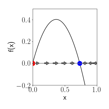
**Figure 2: Graphical analysis of a 1-f dynamical system** Fixpoints are zeros of the function $f(x)$. The red fixpoint is unstable, the blue is stable. Arrows indicate the behavior of $x(t)$ as time progresses.
This is a parabola that opens downwards and crosses the $x$-axis at the fixpoints. Between the fixpoints, in the interval $ (0,\beta / \alpha) $, the parabola $f(x)>0$. Whenever we have an $x(t)$ in that range it will increase until it reaches the fixpoint $x^{\star}=\beta/\alpha$. If on the other we start on the right of that fixpoint the parabola is negative so the change in $x(t)$ is negative and $x(t)$ decreases. This implies that the fixpoint at $\beta/\alpha$ is a stable attractor whereas the fixpoint at $0$ is a repeller. We can visualize this easily by just plotting the function $f(x)$ and observing where it is positive or negative and indicate this by arrows to the right and left, respectively on the $x$-axis, like in Fig. 2.
Graphical analysis
This is a general principle of one dimensional dynamical systems. If we have a dynamical system [ \dot{x}=f(x) ] we can find the fixpoints by finding the solutions to [ 0=f(x) ] which is where the function $f(x)$ crosses the $x-$axis. To investigate the stability we just separate the $x$-axis into regions where $f(x)$ is positive or negative and draw arrows in the respective direction and we immediately see what fixpoints are stable attractors and which ones are not.
We also see an important defining feature of stability. A stable fixpoint is one in which the derivative of $f(x)$ is negative at the fixpoint whereas when $f^{\prime}(x)$ is positive, the fixpoint is unstable. We can check this for the above example [ f(x)=x(\beta-\alpha x) ] for which we compute [ f^{\prime}(x)=\beta-2\alpha x ] at the first fixpoint we find [ f^{\prime}(0)=\beta>0 ] at the second one we find [ f^{\prime}(\beta/\alpha)=-\beta<0 ] which confirms our idea.
**Panel 3: Graphical Analysis: Finding fixpoints and checking their stability.** The function $f(x)=a+bx+cx\^2/2+dx\^3/6$. You can vary the coefficients $a$,$b$,$c$ an $d$. For different values the system can have different sets of fixpoints with different stability properties.
Here's another example: Let's say we have a dynamical system given by [ \dot{x}=a+bx+\frac{1}{2}cx^2+\frac{1}{6}dx^3 ] with four parameters $a$, $b$, $c$ and $d$. Let's assume that the state can be on the entire real axis. Then, depending on the sign and value of the parameters the system can have different sets of fixpoints width different stability properties. You can play with this system in Panel 3. Doing the graphical analysis is much easier than computing the solution analytically. Also, because we are typically interested in the asymptotics only, we don't care about the full solution only in fixpoints, their stability and their basin of attraction if they are attractors. The basin of attraction are the set of initial values for which trajectories approach and attractor.
Marginal stability
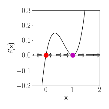
**Figure 3: Marginal Stability**. This happens when $f(x)=f\^\prime(x)=0$.
Here's a situation that isn't generic. Let's say we have a system defined by [ \dot{x}=f(x)=x(x-1)^{2} ] This dynamical system has fixpoints at $x^{\star}=0$ and $x^{\star}=1$. However if we draw $f(x)$ we see that clearly the fixpoint at zero is unstable but what about the other one? Here the function $f(x)$ touches the $x$-axis but doesn't cross it, so the derivative is zero, too. Which means the above conditions aren't telling us anything about the stability. In the graphical analysis we see that in the vicinity of that fixpoint $f(x)>0$ so trajectories will approach the fixpoint from the left but leave it on the right. So the fixpoint is marginally stable.
Example: Epidemics in a population
Let's discuss another example. Let's assume we have a population that is exposed to a transmissable virus. When an individual is infected the virus can be transmitted to another person that is susceptible. Infected individuals remain infectious for some typical time and then become susceptible again.
So first we group individuals into two types, susceptibles and infecteds which we label $S$ and $I$ and we denote the number of individuals in each group by $S(t)$ and $I(t)$ respectively. So we are using the same symbol for the categories and the number of individuals. Let's assume the number of individuals $N$ is fixed, so people don't die or are born. This means that [ N=S(t)+I(t). ] Based on what we said above we have two reactions [ S+I\xrightarrow{\alpha}2I ] and [ I\xrightarrow{\beta}S ] the first being the transmission and the second the recovery. Now let's assume we focus on the population of infecteds. In the time interval $t,t+\Delta t$ each infected can infect a susceptible which increases the number of infecteds. This change should be proportional to the infecteds $I(t)$ because each of them can transmit the disease, and the fraction of susceptible $S(t)/N$ because if a contact occurs an infection only occurs if the other person is susceptible, not if the other person is also infected. The increment due to the first reaction is therefore [ \Delta I_{1}=\alpha IS/N\Delta t ] Likewise, the number of infecteds can decrease because each infected can recover at a rate $\beta$. So the change induced by the recovery is [ \Delta I_{2}=-\beta I\Delta t ] putting these things together we get [ \dot{I}=\alpha IS/N-\beta I ] Now we use the fact that for all times $S=N-I$ so we have a one-dimensional dynamical system: [ \dot{I}=\alpha I(N-I)/N-\beta I ] Now we can simplify this a bit more by defining the fraction of infected individuals [ x=I/N ] to obtain [ \dot{x}=\alpha x(1-x)-\beta x=f(x) ] or [ \dot{x}=x(\alpha(1-x)-\beta x) ] The first thing we see immediately is that $x=0$ is a fixpoint. The other fixpoint is a solution to [ \alpha(1-x)=\beta x ] which solving for $x$ yields [ x^{\star}=1-\frac{\beta}{\alpha}. ] Now because $x$ is by definition a non-negative quantity we see that this fixpoint is only meaningful if [ \alpha>\beta ] which means that the transmission rate must be greater than the recovery rate. The ratio of rates is also known as the basic reproduction ratio [ R_{0}=\frac{\alpha}{\beta} ] and we see from drawing the function [ f(x)=\alpha\left(x(1-x)-\frac{1}{R_{0}}x\right) ] that asymptotically if $R_{0}>1$ the fixpoint $1-R_{0}^{-1}$ is stable and the disease free state is unstable.
If $R_{0}<1$ the disease free state is the only stable fixpoint.
This is also confirmed by a simple agent based simulation depicted in Panel 4. The above model is also known as the SIS-model a well known model in mathematical epidemiology.
An important feature of this model is it's threshold property. The final state of the system is different for different values of $R_0$. The basic reproduction number has to be larger than $1$ in order for the epidemic to become endemic, that is, prevail in the population.
**Panel 2: An epidemic model.** This is an implementation of the SIS model. Infected individuals are shown in red. When they encounter a susceptible (white) an infection can occur. Infecteds recover at the recovery rate. If the transmission rate is too low or the recovery rate is too high, the disease dies out.
Tiny bits of insight
Let's recall briefly the two systems we discussed. we first discussed a particle annihilation / reproduction system governed by the two reactions [ A\xrightarrow{\alpha}2A \qquad A+A\xrightarrow{\beta}\emptyset ] and the dynamical systems [ \dot{x}=x(\alpha-\beta x) ] Secondly, we discussed the epidemic SIS model, governed by the reactions [ S+I\xrightarrow{\alpha}2I\qquad I\xrightarrow{\beta}S ] and the dynamical system [ f(x)=\left(\alpha x(1-x)-\beta x\right) ]
In both systems we have reactions that drive the proliferation of a type of particle of individual, like the reproduction in the first system and the infection the epidemic model, and in both systems we have a self-regulation that inhibits proliferation, like the annihilation reaction in the first system and the recovery in the epidemic system. However, in the first system the proliferation is caused by a single particle and regulation requires an interaction. Whereas in the epidemic model the proliferation requires two particles and the regulation only one.
This yields similar dynamical systems (quadratic functions $f(x)$). However, they are quite different in the dynamics that they induce. The epidemic model exhibits different asymptotics depending on the ratin $\alpha/\beta$. In one regime the epidemic dies out and only for sufficiently large $R_0$ is prevails. Whereas in the reproduction annihilation model, a stable equilibrium is always reached.
This is the sort of insight you can gain from modelling such systems with ODEs.
Oscillatory behavior?
Now, we know from many dynamical phenomena in nature that they can exhibit oscillatory behavior, going up and down increasing at times and decreasing at others. One question is, if we observe a quantity $x(t)$ in a system that goes up an down, if we could model this by a system like [ \dot{x}=f(x). ] It turns out that generically, this doesn't work. For any system like the above, we can only have asymptotic behavior for any initial condition that is either approaching a fixpoint or approaching positive or negative infinity. Why? Let's assume that we have a situation in which $x(t)$ is increasing for some time until a turning point at $t_{0}$ and then decreasing. This would imply that at $t_{0}$ we have $dx/dt=0$ but if that happens we are on a fixpoint to the system would not change anymore by itself. Therefore, if we have a dynamical phenomenon that can be captured by an ODE, we need more than one state variable.
Potentials
Let's look at a general 1-dimensional dynamical system again:
[ \dot{x}=f(x). ] Now imagine that the function $f(x)$ is (minus) the derivative of another function [ f(x)=-dV(x)/dx ] so we can write [ \dot{x}=-V^{\prime}(x) ] If this is the case we can investigate the function $V(x)$ and plug in the solution to the ODE so [ V(x(t)) ] So for every time $t$ we compute the trajectory $x(t)$ plug this into the function $V(x)$ and compute the value. Now if we treat $V(x(t))$ as a function of time, we can compute [ \frac{d}{dt}V(x(t))=\frac{dV(x)}{dx}\frac{dx}{dt}=-(\dot{x})^{2}\leq0 ] This means that if we plot $V(x)$ as a function of $x$ the trajectory $x(t)$ can be visualized as a dot on the function at point $x=x(t)$ and as $x(t)$ evolves it will move on the function $V(x)$ and has to be going downhill until it finds a minimum of $V(x)$ of drift's away to negative infinity. The function $V(x)$ is called a potential. Sometimes it's more intuitive to think of the dynamics evolving in a potential like this.
For example the SIS model that we discusses above with [ \dot{x}=f(x)=\alpha\left(x(1-x)-\frac{1}{R_{0}}x\right) ] is equivalent to [ f(x)=(\alpha-\beta)x-\alpha x^{2} ] has a potential [ V(x)=-\frac{\alpha-\beta}{2}x^{2}+\frac{\alpha}{3}x^{3}. ] This concept can be generalized to more than one dimension and will be very helpful understanding the dynamics of a nonlinear dynamical system. In one dimension this is not telling us too much but in more than one dimension computing such a potential or ``having'' such a potential can be very helpful.
Numerical integration
Given dynamical system $\dot{x}=f(x)$, we can attempt to solve the dynamical system for an initial value $x(t_{0})=x_{0}$ numerically. We split time into little discrete increments of length $\Delta t$, i.e. $t_{n}=t_{0}+n\Delta t$, and $n=0,1,2,....$.Then [ x(t_{0}+\Delta t)=x(t_{0})+\Delta tf(x(t_{0}))+\mathcal{O}(\Delta t^{2}) ] where the last term indicates that we are making an error of the order of $\Delta t^{2}$ if we ignore it. Letting [ x_{n+1}=x_{n}+\Delta t\,f(x_{n})\quad\text{and}\quad x_{0}=x(t_{0}) ] we obtain an approximate solution. This is known as Euler's method. The accuracy is of order $\Delta t$, that means if we for example pick $\Delta t=0.01$ then after $N=100$ steps the error will be or order unity which isn't so good. Much better are Runge Kutta methods, e.g. the second order Runge-Kutta method in which we advance the trajectory based on the dynamics at the midpoint of the interval. Let's call the state at the midpoint $\bar{x}_{n}$ and the dynamics $f(\bar{x_{n}}).$ We then define [ x_{n+1}=x_{n}+\Delta tf(\bar{x}_{n}) ] But how do we find the midpoint? Well, we can't. Only approximately. We advance to the midpoint with ordinary Euler: [ \bar{x}{n}=x{n}+\frac{\Delta t}{2}\,f(x_{n}). ] It's fairly straightforward to show that this method has an accuracy of the order $\Delta t^{2}$ so, again, if we let $\Delta t=0.01$, we could integrate 10000 steps before the algorithm breaks down. Based on the same idea is the algorithm typically used in applications. It's accurate to $4^{th}$ order ($(\Delta t)^{4}$ error) and is called the RK4 (not CR7). The idea is just like the second order RK, building on functional values of many mid points:
[ x_{n+1}=x_{n}+\frac{1}{6}(K_{1}+2K_{2}+2K_{3}+K_{4}) ]
[ K_{1}=f(x_{n})\Delta t ]
[ K_{2}=f(x_{n}+\frac{1}{2}K_{1})\Delta t ]
[ K_{3}=f(x_{n}+\frac{1}{2}K_{2})\Delta t ]
[ K_{4}=f(x_{n}+K_{3})\Delta t ] Now normally, on most programming environments you don't have to implement this yourself because programming packages typically provide this. And not only this but fast algorithms that have fancy things like adaptive stepsize and so forth. To see how easy this this in say python look here: