Two-dimensional Dynamical Systems
In the last few lectures we discussed one dimensional dynamical systems like this one: [ \dot{x}=f(x) ] and learned how to analyze their asymptotics graphically and by calculation. Essentially, this amounted to just plotting the function $f(x)$ and finding the zeros, see One Dimensional Dynamical Systems.
Some 1d-systems were motivated by underlying reaction kinetic cartoons, for example [ X\xrightarrow{\alpha}2X\qquad X+X\xrightarrow{\beta}\emptyset. ] In this particular example, replication (left reaction) and annihilation (right equation) ``compete'' and balance. This example lead to the dynamical system [ \dot{x}=\alpha x-\beta x^{2}=x(\alpha-\beta x) ] for the concentration or abundance of $X$-particles.

**Figure 1:** Schematic of forces in a one-dimensional dynamics system.
We discussed that in systems like this one we can schematically understand the system by a drawing like the one in Figure 1 in which each link indicates the type of influences that play a role. In this case reaction (1) is a positive autocatalytic influence of $X$ onto itself and reaction (2) is an inhibitory influence. Just by looking at the diagram we see that these ``forces'' can balance yielding a stable equilibrium.
If we look at a different dynamical system, for instance [ 3X\xrightarrow{\alpha}4X\qquad X\xrightarrow{\beta}\emptyset ] with a corresponding dynamical system [ x=x\left(\alpha x^{2}-\beta\right) ] we see that it is structurally is different. However, schematically, it looks the same, we have a reaction that is a positive influence (1) and increases the abundance, and another equation (2) that decreases it. And also here we can expect a balancing scenario in which both reactions stabilize the system.
Sometimes, we can already see what to expect from a dynamical system just by drawing the schematics. This is even more powerful in 2D where analytic treatments are often much harder and developing an intuition for the dynamics even more vital.
Basics
Now we will discuss two dimensional dynamical systems. Don't worry, we won't be increasing dimensionality step by step to discuss peculiarities of each of the dimensions. We will only discuss two dimensions in more detail because even higher dimensional systems can sometimes be understood by putting 2D-motifs together that are derived from 2D-interactions. We'll discuss this in more detail later.
A two dimensional system's state is defined by two dynamic variables, usually denoted by $x$ and $y$ so the state is the pair: [ \mathbf{r}(t)=\left(x(t),y(t)\right). ] As you may expect, we will be discussing systems that are defined by [ \dot{x} =f(x,y) ] [ \dot{y} =g(x,y), ] so by two functions $f$ and $g$ that define how each component of the state changes. A more compact notation is this one [ \mathbf{\dot r}=\mathbf{f}(\mathbf{r}) ] where the $\mathbf{r}(t)$ is a 2D state-vector and a state-dependent vector [ \mathbf{f}(\mathbf{r})=\left(f(x,y),g(x,y)\right) ] that tells us how the state changes in every state $\mathbf{r}$. This notation becomes more practical in higher dimensions. For 2D we can stick with the explicit notation for each component using $x$ and $y$. If we visualize the state-space as the $x-y-$plane, then we can think of $\mathbf{f}(\mathbf{r})$ as little vectors defined at every location which is why this is called a vector-field. We'll discuss this in more detail below.
An example
First let's derive a 2D dynamical system using reactions and schematics. Let's say we have two different types of particles, $A$ and $B$ and they interact with each other and with themselves according to four reactions like so:
[ A\xrightarrow{\alpha}2A \qquad A+A\xrightarrow{\beta}A ]
[ B\xrightarrow{\gamma}\emptyset\qquad A+B\xrightarrow{\delta}2B ]
**Panel 1:** In this agent based simulation two types of particles ***A*** (white) and ***B*** (red) interact. The whole system is governed by the reactions: $A\xrightarrow{\alpha}2A$, $A+A\xrightarrow{\beta}A$, $B\xrightarrow{\gamma}\emptyset$ and $A+B\xrightarrow{\delta}2B$. Vary the parameters and try to find a regime in which the abundance of particles varies for long times. Before you change parameters, give the system some time to evolve.
Let's denote the concentration of $A$ and $B$ by $x$ and $y$, respectively. Then we know that reaction (1) above replicates $A$ and therefore increases $x$ by a term $\alpha x$. The second equation models a collision of $A$'s by which one agent is destroyed, so this is a term $-\beta x^2$. The third reaction decrease $B$ by spontaneous disappearance so we have a terms $-\gamma y$ by which $y$ change accordingly.
The interesting equation is (4) which is a two particle reaction of $A$ with $B$ that both decreases $x$ and increases $y$ by a factor $\delta xy$. So, all in all we get a dynamical system

**Figure 2:** Interactions of the system: $\dot{x} =\alpha x-\delta xy-\beta x^2$ and $\dot{y} =\delta xy-\gamma y$.
[ \dot{x} =\alpha x-\delta xy-\beta x^2 ] [ \dot{y} =\delta xy-\gamma y ] Schematically we see that $A$ is self-reinforcing, both $A$ and $B$ have an inhibitory impact on themselves (reactions (2) and (3)). The interesting part is the interaction that is both, a positive impact of $A$ onto $B$ and a negative impact of $B$ onto $A$ which is driven by the last reaction. So, the interaction is of opposite sign in a way. Figure 2 illustrates the schematic diagram for this system.
Schematic analysis
In the example above we didn't do much, except made a little schematic. We can do more. We can compute fixpoints, their stability and gain an overall understanding of the behavior and of the asympotics of a system. Below is a recipe on how to investigate a system like the example system above. Before we do this for some examples let's see however what kind of qualitatively different schematics we can have in a 2D-system.
Mutual Inhibition
Let's look at these reactions
[ \emptyset \xrightarrow{\alpha}A \qquad A \xrightarrow{\beta}\emptyset ]
[ B \xrightarrow{\gamma} 2 B \qquad 3B \xrightarrow{\delta}2B ]
[ A+B\xrightarrow{\xi}\emptyset ]
The first two equations alone yield a dynamical systems [ \dot{x}=\alpha-\beta x ] so just these two would imply a self-regulating $A$ population by spontaneous creation of $A$'s (reaction 1) and spontaneous death (reaction 2). So by itself we have something that calls for an equilibrium in which both reactions balance. In fact, this is what you get if you just have $A$'s. If we only focus on $B$ reactions (3) and (4) we get [ \dot{y}=\gamma y-\delta y^{3}. ] Again a system in which two ``forces'' of opposite sign balance. The interesting stuff is happening because of equation (5) which implies a negative change of both $A$ and $B$ proportional to $-\xi xy.$ This couples the system and we get
[ \dot{x} =\alpha-\beta x-\xi xy ] [ \dot{y} =\gamma y-\delta y^{3}-\xi xy ] Unlike the system above, schematically we see a system in which the interaction is mutually inhibitory.

**Figure 3:** Mutual Inhibition.
So by looking at the corresponding schematic in Figure 3 we can imagine that in such a scenario we could have an asymptotic state in which either $A$ and $B$ ``win'' and push the competitor to zero, or we may expect that for a low value of $\xi$ in a regime of weak inhibition that both $A$ and $B$ approach a non-zero stable state each.
You can investigate and confirm this conjecture using the Interactive tool for 2D systems in the Script Collection. In the tool, choose the Mutual Inhibition system and tune the parameters to generate a stable coexistence state for some set of parameters, and try to find conditions for a winner takes it all scenario.
Cooperative systems
Sometimes, we obtain the ODEs defining a dynamical system or a model in a different way, e.g. a book, or a paper and it helps reading a schematic interaction off the equations defining the system. Consider this system [ \dot{x} =r_{1}x(1-x)-x+\alpha xy(1-y) ] [ \dot{y} =r_{2}y(1-y)-y+\beta yx(1-x) ] defined for $x,y\geq\text{0}$ and say for parameters $0\leq r_{1/2}<1$. Let's clarify this equation a bit and write it as:
[ \dot{x} =r_{1}\,\lambda(x)-x+\alpha x\,\lambda(y) ] [ \dot{x} =r_{2}\lambda(y)-y+\beta y\,\lambda(x) ] where the function [ \lambda(z)=z(1-z) ] is the typical, self-regulated logistic growth function that is linear for low concentrations and has the limiting $1-z$ factor. We see that the interaction is hidden in the last terms of the rhs of the two parts of the system and controlled by the two parameters $\alpha$ and $\beta$. Without the interaction terms each of the systems is equivalent to the epidemic SIS system with a subcritical reproduction number (see Script on One-Dimensional Dynamical Sysems). So for instance if $\alpha=0$ the first equation is [ \dot{x}=r_{1}\,x(1-x)-x ] that only has the $x=0$ state as a stable fixpoint (because we say that $r_{1}<1$) and likewise for $y$ if $\beta=0$. Now let's look at what the term $\alpha xy(1-y)$ does. Well this term is positive so it's a cooperative influence of $y$ onto $x$. But it's limited if $y$ gets too large the factor $1-y$ makes sure the cooperativity is clamped. The same is true the other way around. The term $\beta yx(1-x)$ represents a positive effect of $x$ onto $y$. So if we were to draw a schematic we have a system in which each element is doing the usual self-excitation with saturation, and additional negative self-loop but a positive interaction like so:

**Figure 4:** Cooperation of two replicating and self-regulating elements.
A system like this is mutually cooperative. The questions now are: What is the asymptotic behavior of the system? Is the cooperativity strong enough to stabilize a stationary state in which both $x$ and $y$ are non-zero? Is the $x=y=0$ state always stable? Do we have states in which only one species is stabilized by the other, but not vice versa?
You can see for yourself using the Interactive tool for 2D systems again. In the systems menu pick Cooperative System. It turns out it can can up to 5 different stationary states and three stable coexistence states. Try to find conditions for it.
Activator-inhibitor systems
The first example we discussed and schematically analyzed is an example of an activator-inhibitor system in which one element inhibits the other and the other activates the first. These systems are defined by an asymmetric coupling. One of the more famous systems that captures activator-inhibitor dynamics is a predator-prey model known as the....
...Lotka Volterra model
This is defined by the equations
[ \dot{x} =x(\alpha-\beta y) ] [ \dot{y} =y(\gamma x-\delta) ] for the abundance $x$ and $y$ of two species $A$ and $B$ respectively. Species $B$ inhibits $A$, see the term $-\beta xy$. The reproduction of $B$ increased by the abundance of $A$, see the term $\gamma xy$. Therefore, $A$ must be the prey that get consumed by the predator $B$. In addition to the interaction terms we have regular replication in the prey (the term $\alpha x$) and decay in the predator $-\delta y$. This therefore follows a similar schematic as shown in Figure 2. Note, however, that in the absence of the predator, prey will grow exponentially without bounds, so the LV-system makes no sense in this marginal case. Something to keep in mind.
In an activator-inhibitor system like this one, we can imaging that the interaction of activation and inhibition can generate a stable state in which both effects balance. But we can also imagine that the system cycles through phases:
- If both predator ($y$) and prey ($x$) are low, $x$ can exponentially increase.
- After that, the predator abundance can pick up because at some point there's sufficient prey to consume.
- The increase in predators will decrease in prey until ...
- .... there's not enough prey and the predator population will decrease again because there's not enough food, yielding situation 1.
We see just by this train of thoughts that we can expect activator-inhibitor systems to exhibit cyclic solutions.
Analysis
One way of investigating 2D systems is of course just by plotting $x(t)$ and $y(t)$ for an initial condition $x(0)$ and $y(0)$ as a function of $t$. But just like in 1D systems, if we are more interested in the asymptotics, it's more helpful to visualize the trajectory in phasephase, sometimes called state-space, which is the 2D $x-y$-plane. The initial condition is just a location in this space, and the solution ($x(t),y(t)$) is a path in it. Irrespective of what this solution looks like we can deduce a few things that must hold. For example, trajectories can't cross. If this were possible, the solution would not be unique at the intersection. It wouldn't know where to go.
The flow field
As mentioned above we should think of a 2D system as a vector-field, so at every position ($x,y$) in state-space we imagine a vector [ \left(f(x,y),g(x,y)\right) ] Because in the dynamical system the components of this vector represent the change of $x$ and $y$ the vectors point in the direction of motion. Now we can put a grid across a region of state-space and at each grid point draw a vector. This is difficult to do by hand, but computers can do this very quickly. See Panel XX. In the panel the, the flow field of the cooperative system
[ \dot{x} =r_{1}\,x(1-x)-x+\alpha x\,y(1-y) ] [ \dot{y} =r_{2}y(1-y)-y+\beta y\,x(1-x) ] is shown for $r_{1}=0.1$, $r_{2}=0.1$, $\alpha=3.974$ and $\beta=4.641$ .
**Panel 2:** Flow field of the cooperative system above. At each point, a flow-vector indicates the direction of motion of the state of the system. **Hover** with a mouse to see a full trajectory that starts at the location of the mouse. **Click** so make a chosen trajectory stick. The button wipes the saved trajectories.
Just by looking at the little vectors we see that potentially the system has 3 attractors which are points in state-space. In the panel you can move the mouse across the state-space and for an initial condition ``under the mouse pointer'' a full trajectory is computed. When you click you can freeze it and select another one. Try it.
Asymptotics Brainstorm
We are almost ready to do some math. But before we do, let's take the previous example and discuss what we could expect from a 2D dynamical system when we think of asymptotics.
Well, we could have points as attractors, fixpoints in 2D. So points like $(x^{\star},y^{\star})$ that not only fulfill [ f(x^{\star},y^{\star})=g(x^{\star},y^{\star})=0 ] but that also attract trajectories. In the example above we observe three of those attractive fixpoints and depending on the initial condition different trajectories will approach one or the other fixpoint.
We can also think of other types of attractors in 2D. In two dimensions we can imaging that trajectories can be closed loops, cyclic solutions such that [ x(t) =x(t+T)\qquad y(t) =y(t+T) ] for any point on the cycle and $T$ being the time it takes to go around. This is the sort of thing we expect for activator-inhibitor systems. And in fact we will discuss and analyze a specific example of this. You can sneak-peak in the Examples of 2D Dynamical Systems - Interactively - Script and see that the Lotka-Volterra system actually exhibits a family of such periodic orbits around one of its fixpoints.
Poincare-Bendixon Theorem
In addition to this we could have trajectories that explode to $\pm\infty$. Let's exclude this for a second and assume that we can define a region in state-space for which we can show that the flow enters the region everywhere on its boundary. What can we say about trajectories that enter that region. For sure there could be an attractive fixpoint in the region that attracts all trajectories that enter the region. We could also have a limit cycle, a periodic solution that attracts all the trajectories, see for example the Brusselator or Predator Prey system in the Examples of 2D Dynamical Systems - Interactively - Script . But could we also have something like a trajectory that folds up infinitely many times like illustrated in Figure 5?

**Figure 5:** Asymptotics in a 2D dynamical systems are restricted by the Poincare-Bendixon Theorem.
Could we have a trajectory that folds itself ad-infinitum, never crossing but getting folded closer and closer? In principle this should be possible. But it turns out that a deep mathematical theorem known as the Poincare-Bendixon theorem states that in 2D this isn't possible. So all we are left with as asymptotic behaviors are periodic cycles or stable fixpoints (potentially infinitely many, though). This limits the variety of possibilities immensely. The Poincare-Bendixon Theorem is only true for 2D. When we have an additional dimension, we can have bounded solutions that are neither periodic not fixed. We can have what is known as strange attractors. These objects are very weird and play a role in deterministic chaos.
Fixpoints and nullclines
Now let's dig into 2D systems a bit deeper. Given a system we usually follow a recipe. First, just like in 1D we try to find the systems fixpoints. These are all the points in state-space for which
[ \dot{x} =f(x,y)=0 ] [ \dot{y} =g(x,y)=0 ] Let's do this for the Lotka-Volterra system: [ \dot{x} =x(\alpha-\beta y) ]
[ \dot{y} =y(\gamma x-\delta) ]
This yields the trivial fixpoint [ x^{\star}=y^{\star}=0 ] and the second fixpoint [ (x^{\star},y^{\star})=(\delta/\gamma,\alpha/\beta) ] First thing we do is draw those in the state space. For the Lotka-Volterra system we are only interest in the upper-right quadrant of the $x-y-$plane, i.e. the region for which $x\geq0$ and $y\geq0$.
The next thing we do is draw the nullclines. The $x$-nullcline is defined by all the points that fulfill [ f(x,y)=0 ] Usually this is a set of simple curves defined in state space. For the LV-system the $x-$nullclines are the points defined by $x=0$ which is the $y$-axis and the horizontal line [ y=\alpha/\beta ] Because $\dot{x}=0$ on these curves the trajectories of the LV system must cross the $x-$nullcline vertically, i.e. parallel to the $y$-axis. The $x$-nullclines also separate the state-space into regions where $\dot{x}>0$ (below the nullcline $\alpha/\beta$) and where $\dot{x}<0$, above that line. Likewise the $y$-nullclines are given by the $x-$axis (where $y=0$) and the vertical line $x=\delta/\gamma$. The trajectories of the system have to cross the $y$-nullcline horizontally. The $y$-nullcline separates the state-space into regions where $\dot{y}>0$ and $\dot{y}<0$.
Fixpoints are obviously the intersections of $x$- and $y$-nullclines. For the Lotka-Volterra system we can separate the state-spaces into four region in which the sign of the rate of change $\dot{x}$ and $\dot{y}$ are different. So here we have 4 regions:
- A: $\dot{x}<0$ and $\dot{y}<0$ so trajectories point south-west
- B: $\dot{x}>0$ and $\dot{y}<0$ so trajectories point south-east
- C: $\dot{x}>0$ and $\dot{y}>0$ so trajectories point north-east
- D: $\dot{x}<0$ and $\dot{y}>0$ so trajectories point north-west
So by drawing little arrows in these directions we can get a sense of the trajectories. It looks like that, as expected for an activator-inhibitor system that the trajectories circle around the fixpoint. This is also clear from looking at the flow-field.
All of this is information is collected in Figure 6.
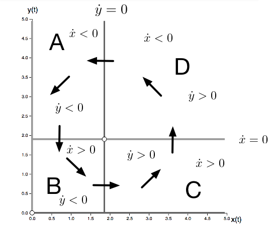
**Figure 6:** A guess at the dynamics of the Lotka-Volterra system. $x$-nullclines are shown in light grey, $y$-nullclines in dark grey. The nullclines separate state-space into four region in which trajectories must move into one of the four direction NW,NE, SE, SW.
One of the things we cannot say here whether the circular movement in state-space will spiral down to the fixpoint in the center, or spiral outwards or generate concentric periodic orbits or potentially have a limit cycle. It turns out that for the LV system, we can show that all the orbits are periodic, the shape depending on the initial condition. You can check this again here.
Fixpoint stability
To get a bit more information about a system we can study the behavior of a system near its fixpoints. Remember that in 1D $\dot{x}=f(x)$ with a fixpoint at $x^{\star}$ it was sufficient to look at the derivative at the fixpoint $df(x)/dx\,|\,x=x^{\star}$. Likewise in a 2D system, we can linearize the system around the fixpoint, Let's say [ x(t) =x^{\star}+\delta x(t) ] [ y(t) =y^{\star}+\delta y(t) ]
where $\delta x,\delta y$ terms are small deviations from the fixpoint. So this yields [ \dot{\delta x} =\dot{x}=f(x^{\star}+\delta x(t),y^{\star}+\delta y(t)) ] [ \dot{\delta y} =\dot{y}=g(x^{\star}+\delta x(t),y^{\star}+\delta y(t)) ] which is approximately [ \dot{\delta x} =\dot{x}\approx f(x^{\star},y^{\star})+ \frac{\partial f(x^\star,y^\star)}{\partial x}\delta x + \frac{\partial f(x^\star,y^\star)}{\partial y}\delta y ] [ \dot{\delta y} =\dot{y}\approx g(x^{\star},y^{\star})+ \frac{\partial g(x^\star,y^\star)}{\partial x}\delta x + \frac{\partial g(x^\star,y^\star)}{\partial y}\delta y ] The first terms in each equation are zero. So we can write this compactly as
$$ \dot{\left(\begin{array}{c} \delta x\\ \delta y \end{array}\right)}=\mathbf{J}(x^{\star},y^{\star})\left(\begin{array}{c} \delta x\\ \delta y \end{array}\right) $$
where the matrix $\mathbf{J}$ is the Jacobian, the matrix of partial derivatives at the fixpoint
$$ \mathbf{J}(x^{\star},y^{\star})=\left(\begin{array}{cc} \partial_{x}f & \partial_{y}f\\ \partial_{x}g & \partial_{y}g \end{array}\right)_{(x,y)=(x^{\star},y^{\star})} $$
Now it turns out that the stability of the fixpoint is determined by the eigenvalues of the Jacobian. This is why. The dynamics for the variables $\delta x$ and $\delta y$ is linear and has the form
[ \dot{\mathbf{x}}=\mathbf{A}\mathbf{x} ]
if we write the two component vector compactly as $\mathbf{x}$ and $\mathbf{A}$ is a $2\times 2$ matrix
$$ \mathbf{A}=\left(\begin{array}{cc} a & b\\ c & d \end{array}\right) $$
A solution to the above system is (generically) given by
[ \mathbf{x}(t)=c_{1}\mathbf{v}_{1}e^{\lambda_{1}t}+c_{2}\mathbf{v}_{2}e^{\lambda_{2}t} ]
where $c_{1/2}$ are constants, $\mathbf{v}_{1/2}$ the eigenvectors of $\mathbf{A}$ and $\lambda_{1/2}$ the eigenvalues.
Also, if your imagine that $\mathbf{A}$ has two different and linearly independent eigenvectors $\mathbf{v}_{1}$ and $\mathbf{v}_{2}$ pointing in some direction and if you start your system on the line that is spanned by an eigenvector the trajectory will stay on it.
So along that line the system behaves like a one-dimensional system. And we can have different combinations of stable or unstable lines that are spanned by the two eigenvalues. So just by this reasoning we can expect three different scenarios, see Figures 7-9.
The situation is a bit complexified by the fact that the eigenvalues and eigenvectors of a general $2\times 2$ matrix can be complex numbers like $z=\alpha+i\beta$ where $i^2=-1$ is the imaginary unit. If you investigate linear systems comprehensively you can dig into this and classify all possible types of behaviors of linear systems. What matters here is that we can see that the asymptotic behavior is generically dominated by the real part of the eigenvalues. We can see already that if one of the real parts is positive one of the terms will explode to infinity which means that the fixpoint is unstable. Stability requires that the real part of both eigenvalues are non-positive.
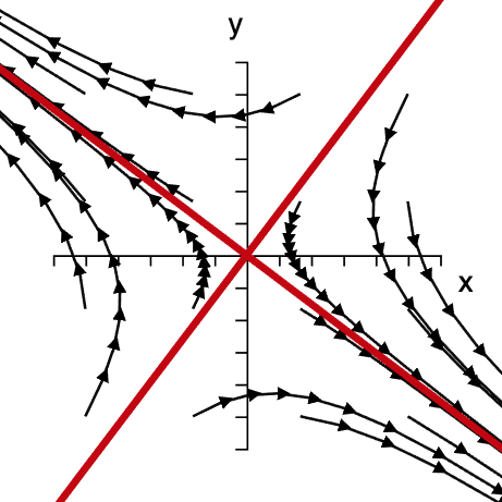
**Figure 7: The saddle node.** If $\lambda_1>0$ and $\lambda_2<0$ trajectories in the vicinity of the fixpoint are attracted along one eigenvector and repelled by the other. This implies that generically all trajectories are eventually moving away from the fixpoint.
Without going into the dynamics of linear systems too deeply, let's briefly summarize what can happen. To this end we need to compute the eigenvalues of a general $2\times 2$ matrix. These can be expressed in terms of the trace $s$ and the determinant $\Delta$ of the matrix which are defined as [ s =a+d ] [ \Delta =ad-bc ] The eigenvalues are then [ \lambda_{1/2}=s/2\pm \left(s^{2}/4-\Delta \right)^{1/2} ] It's good practice to check this. We can now classify different situation.
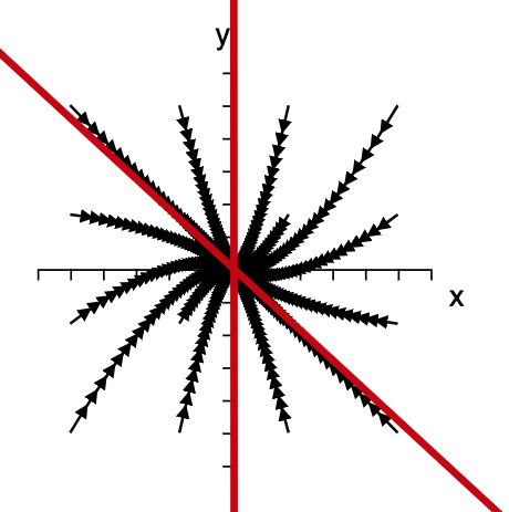
**Figure 8:** If $\lambda_1,\lambda_2<0$ trajectories in the vicinity of the fixpoint approach it The red lines are each spanned by one of the eigenvectors of the $2 \times 2$ matrix $\mathbf{A}$.
Saddle nodes: $\Delta<0$
In this case both eigenvalues are real, one is negative one is positive. This means the fixpoint is a saddle with one direction that is attractive and one direction that is repelling. Trajectories around such a fixpoint look like the ones in .
Stable node: $s^{2}/4>\Delta>0$ and $s<0$
In this case both eigenvalues are real and smaller than zero. So we have two directions that are both attractive. and all initial conditions in the vicinity of the fixpoint will move towards it.
Unstable node: $s^{2}/4>\Delta>0$ and $s>0$
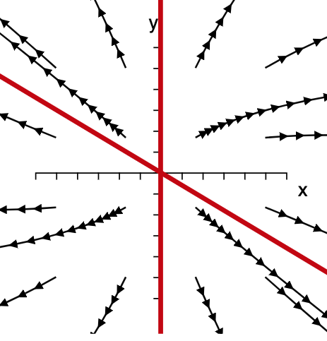
**Figure 9:** If $\lambda_1,\lambda_2>0$ trajectories in the vicinity of the fixpoint are repelled by it. The red lines are each spanned by one of the eigenvectors of the $2 \times 2$ matrix $\mathbf{A}$.
In this case both eigenvalues are real and larger than zero. So we have two directions that are both repulsive. All initial conditions in the vicinity of the fixpoint will move away from it.
Stable spiral: $\Delta>s^{2}/4$ and $s<0$
Because of the first condition, the eigenvalues are complex and also complex conjugates of each other. [ \lambda_{1/2}=s/2\pm i(\Delta-s^{2}/4)^{1/2} ]
**Panel 3:** Linearized dynamics near a fixpoint. The sliders modify the four elements of the $2\times 2$ matrix. In response to this the trace $s$ and determinant $\Delta$ of the matrix and thus the eigenvalues change. The red lines indicate the eigenvector spaces if the eigenvalues are real.
This implies an oscillatory component of the solution. The term under the root is the angular frequency with with a solution oscillates around the fixpoint. Because of $s<0$ the trajectories approach the fixpoint and it is therefore a stable spiral.
Unstable spiral: $\Delta>s^{2}/4$ and $s>0$
This is just the opposite scenario. We still have a spiral but it expands outwards and is an unstable spiral.
Focus: $s=0$ and $\Delta>s^{2}/4$
In this case the eigenvalues are purely imaginary and trajectories of the linear system are periodic orbits that cycle around the fixpoint.
This is a non-comprehensive list of behaviors, there are other special cases for instance when $\Delta=s^{2}/4$ or $\Delta=0$.
In Panel 3 you can vary the elements $a$, $b$, $c$ and $d$ of the matrix $\mathbf{A}$ and inspect the behavior of a dynamical system near a fixpoint.
Memorize this:
It's a good idea to memorize Figure 10 that compiles the different situations:
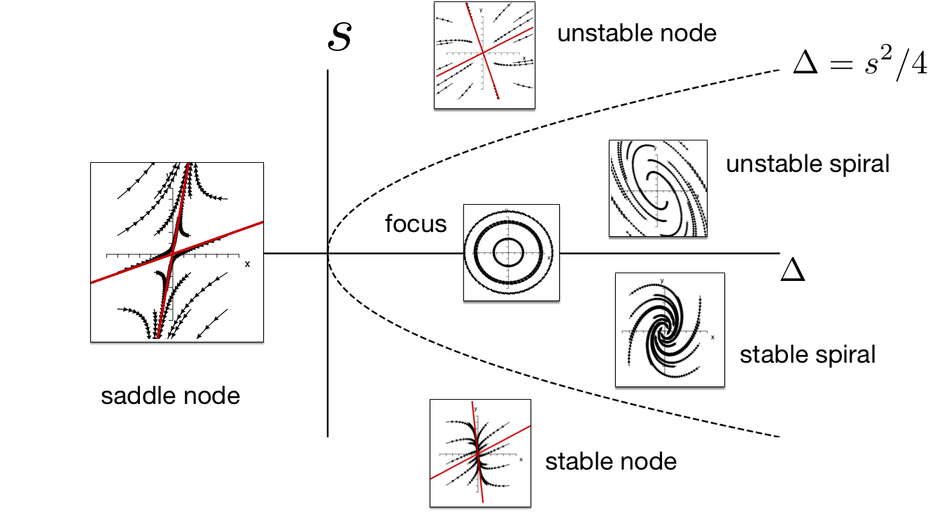
**Figure 10: Classification of dynamics near a fixpoint** For different combinations of trace $s$ and determinant $\Delta$ of the Jacobian at the fixpoint we see different types of behavior. A fixpoint is only asymptotically stable if $s<0$ and $\Delta >0$.
WLet's apply what we discussed to the following example:
The Duffing Oscillator
Consider the following dynamical system: [ \dot{x} =y ] [ \dot{y} =-y+x-x^{3} ] This one is known as the Duffing oscillator. It describes the motion of a simple, damped mechanical system that is subject to a nonlinear force. Let's say we have a simple mechanical problem, e.g. a particle of mass $m$ at position $x$ that is subject to a force $F(x)=x-x^{3}$ and a frictional force that is speed dependent $F_{f}=-\gamma v$. We use Newton's second law [ F=ma ] and get [ m\ddot{x}=x-x^{3}-\gamma\dot{x} ] Now this is a one-dimensional system but the dynamical equation involves a second derivative with respect to time. We can also write this as [ \dot{x} =y ] [ m\dot{y} =x-x^{3}-\gamma y ]
identifying the speed $v$ as a second variable. So effectively we have a two-dimensional system of first order. Now if we, for simplicity let $m=1$ and $\gamma=1$ we recover the equations above. We can investigate this system in the usual way, computing the fixpoints, the nullclines plotting the flow etc.. Again, you can try this using the interactive tool. This suggests that we have three fixpoints the trivial one at $(0,0)$ and the two fixpoints at $(\pm1,0).$ The interactive tool suggests that the latter two are stable spirals and the central one is unstable. Let's see if linear stability analysis confirms this observation. We first compute the Jacobian
$$ \mathbf{J}(x^{\star},y^{\star})=\left(\begin{array}{cc} 0 & 1\\ 1-3x^{2} & -1 \end{array}\right) $$
Now let's look at the fixpoint $(0,0)$ for which we have
$$ \mathbf{J}(0,0)=\left(\begin{array}{cc} 0 & 1\\ 1 & -1 \end{array}\right) $$
which yields $s=-1<0$ and $\Delta=-1<0$. We therefore have an unstable saddle with a positive and negative direction. Now at the other two fixpoints we have
$$ \mathbf{J}(\pm1,0)=\left(\begin{array}{cc} 0 & 1\\ -2 & -1 \end{array}\right) $$
which gives $s=-1$ and $\Delta=2>s^{2}/4$ so we have two stable spirals which we expected.
Asymptotics of the Lotka-Volterra system
Let's do the same for the Lokta-Volterra System:
[ \dot{x} =x(\alpha-\beta y) ] [ \dot{y} =y(\gamma x-\delta) ]
Here we are interested in the stability of the fixpoint $(\delta/\gamma,\alpha/\beta)$. The Jacobian is given by
$$ \mathbf{J}(x^{\star},y^{\star})=\left(\begin{array}{cc} \alpha-\beta y & -\beta x\\ \gamma y & \gamma x-\delta \end{array}\right) $$
At the fixpoint we have
$$ \mathbf{J}(\delta/\gamma,\alpha/\beta)=\left(\begin{array}{cc} 0 & -\beta\delta/\gamma\\ \gamma\alpha/\beta & 0 \end{array}\right) $$
So the trace is $s=0$ and $\Delta=\alpha\delta$ so we are dealing with a focus. This is interesting. However, unlike some of the other behaviors, this is a behavior that is structurally unstable. Imagine that in addition to the above rhs. of the equations we have a small term
[ \dot{x} =x(\alpha-\beta y)-\epsilon ] [ \dot{y} =y(\gamma x-\delta) ]
This wouldn't change the fixpoint substantially but would imply a negative trace and the focus is replaced by an inward spiral.