Binning and sampling

Temporal networks are, naturally, objects recorded in a world of continuous time. However, more often than not, real-world temporal network data are supplied in discrete time format. These formats typically have two interpretations.

Binning

In data recorded in real experiments, an edge is often described as a pair of time \(t=n\Delta t\) and edge \((i,j)\) which typically means that this edge was active at some time in the interval \([n\Delta t,n\Delta t+\Delta t)\) (in some cases it means it was active at some time in the interval \([n\Delta t -n\Delta t,\Delta t)\). However, in subsequent analyses, the edge is typically treated as present in the whole interval. This means that the duration of edges is extended to both ends of a time interval, a procedure we will call binning in the following.

A consequence of binning is that the number of observed edges at any time is systematically greater than or equal to the actual number of edges. Nodes switching between groups in one time bin might further produce a single artificially large group. However, all edges active in the experiment are also reflected in the data.

In tacoma, binning is done using tacoma.api.bin().

# 5 minutes interval binning of network with time_unit='s'
binned_temporal_network = tc.bin(temporal_network, dt = 300.0)

# binning to 6 time steps (6 bins)
binned_temporal_network = tc.bin(temporal_network, N_time_steps = 6)

The binning procedure is visualized in the following figure.

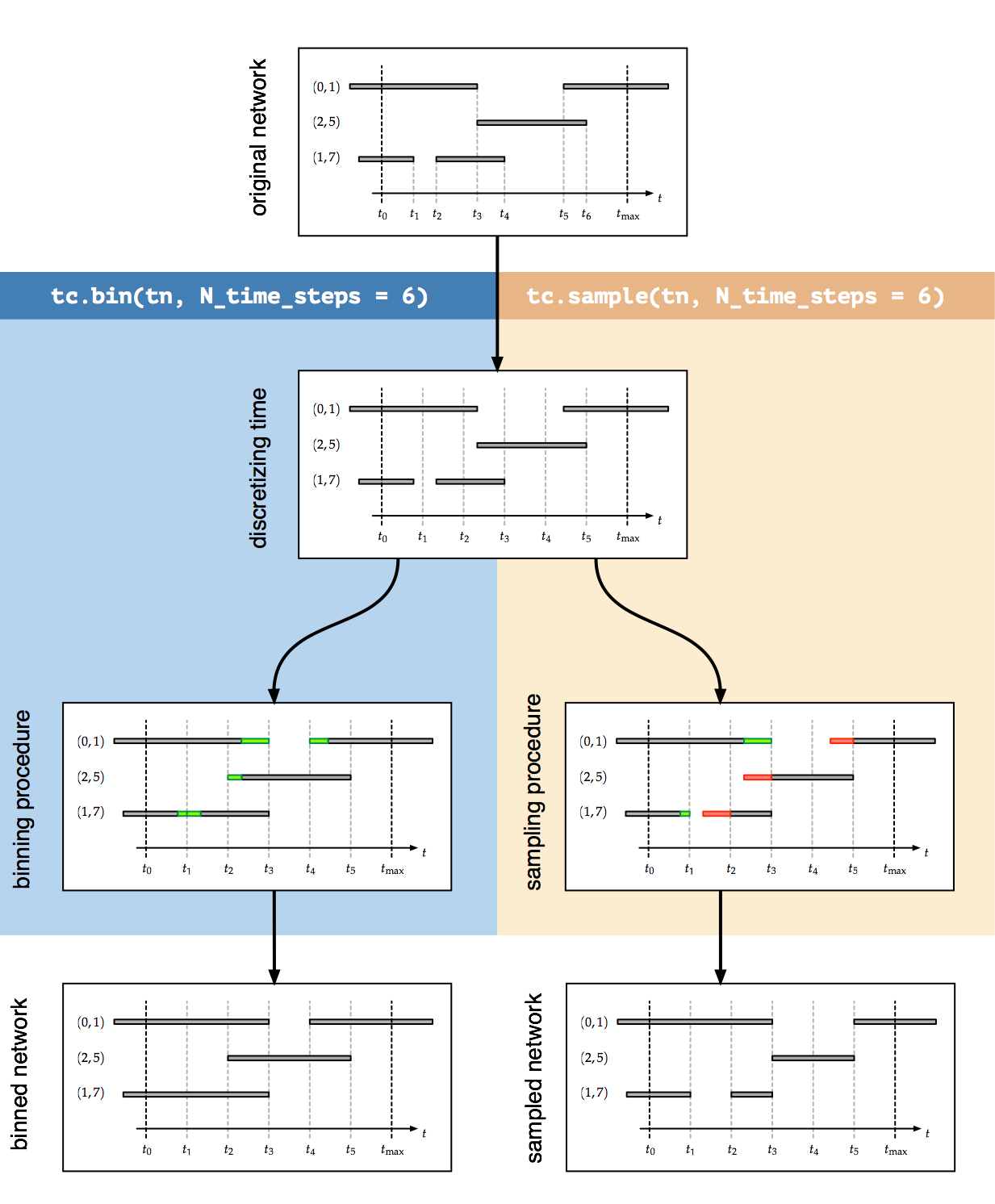
Binning and sampling.

Sampling

Sometimes, data given as a pair of time \(t=n\Delta t\) and edge \((i,j)\) means that at that certain time, an edge was active. Since we do not know anything about the duration of the edge, we have to assume it is active until the end of the interval.

A consequence of sampling is that edges existing at a certain time, typically became active in the predecessing time interval. Hence, duration is shortened in the beginning of an active edge. Furthermore, we have to assume that the edge is active until the end of the interval and thus, its duration is lengthened towards the end (see Figure above). Edges being switched on and switched off within the same time interval are not reflected in the data, at all, meaning that paths for the spread of information are possibly deleted.

In tacoma, sampling is done using tacoma.api.sample().

# 5 minutes interval sampling of network with time_unit='s'
sampled_temporal_network = tc.sample(temporal_network, dt = 300.0)

# sampling at 6 times including t0
sampled_temporal_network = tc.sample(temporal_network, N_time_steps = 6)

Applications

Obviously, both approaches have their downsides and transform the data in a way such that information is lost. If avoidable, data should neither be binned nor sampled. However, some algorithms might only be applicable for discrete-time data. Furthermore, models operating in continuous time have to be compared to real-world data supplied in discrete time and thus have to be either binned or sampled.