Introduction to Complex Systems
This is the collection of slide decks that supplement the material for the course Introduction to Complex Systems.
Synchronization
Christiaan Huygens (1629 – 1695)
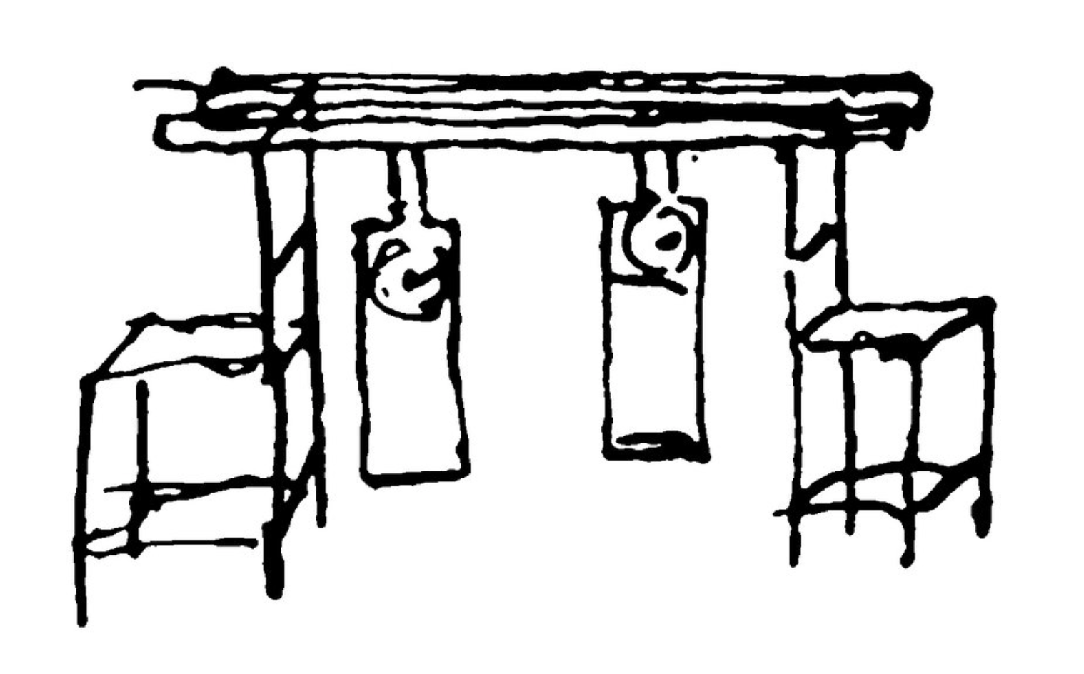
Huygens noticed that two mechanical clocks when attached to a beam synchronize the movement of their pendula. Even when perturbed, the clocks return to the sychronous state.
Christiaan Huygens (1629 – 1695)
It is quite worth noting that when we suspended two clocks so constructed from two hooks imbedded in the same wooden beam, the motions of each pendulum in opposite swings were so much in agreement that they never receded the least bit from each other and the sound of each was always heard simultaneously. Further, if this agreement was disturbed by some interference, it reestablished itself in a short time. For a long time I was amazed at this unexpected result, but after a careful examination finally found that the cause of this is due to the motion of the beam, even though this is hardly perceptible
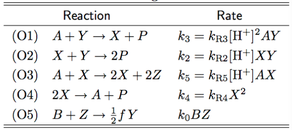
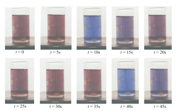
Belousov–Zhabotinsky reaction
The BZ reaction is an activator-inhibitor systems that exhibits oscillatory behavior in a well mixed container
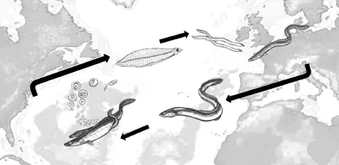
Eels (Anguilla anguilla)
The migration routes of the European eel
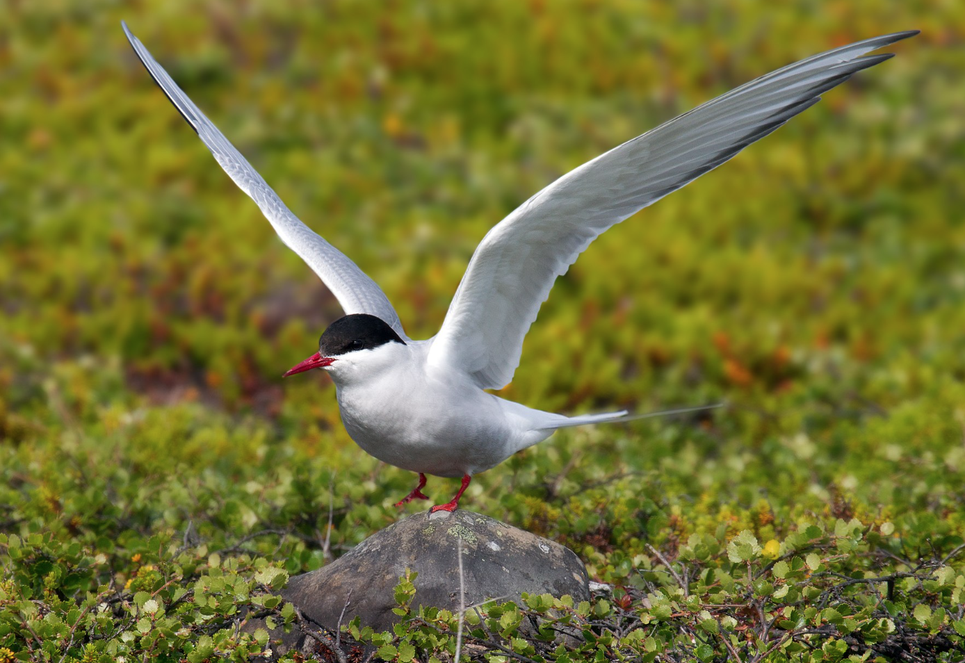
Arctic tern (Küstenseeschwalbe)
The arctic tern likes the sun, and likes it cold, so every year it migrates from the arctic to the antarctic. Twice.
The tern sees more sun than any other organsism on the planet.
On average a tern flies a distance of 70,000 km each year.
Two insect species
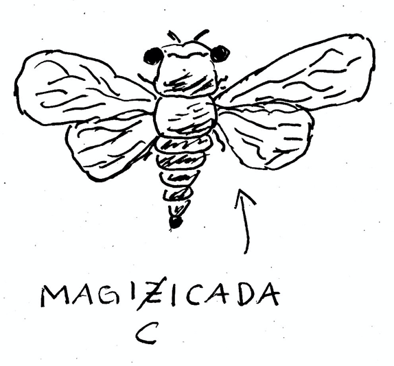
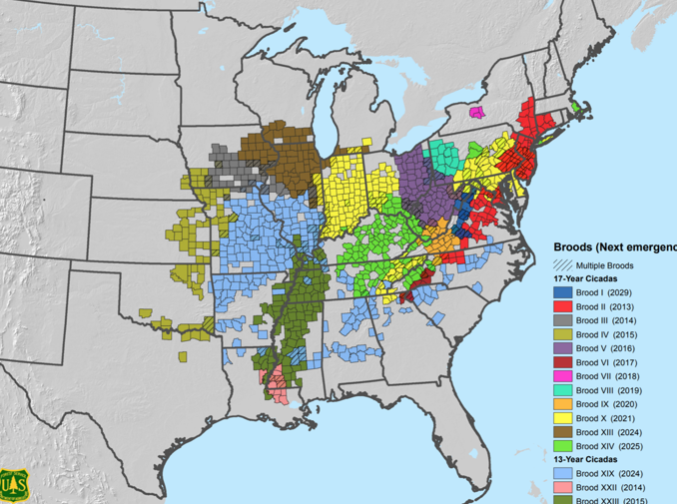
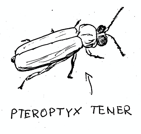
Two insect species
More examples
Measles Dynamics in the UK
- Annual/biannual cycles of measles cases in the UK
- an example spatial synchronization
- Grenfell, B. T., Bjørnstad, O. N. & Kappey, J. Travelling waves and spatial hierarchies in measles epidemics. Nature 414, 716
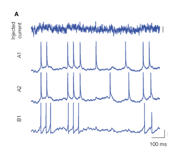
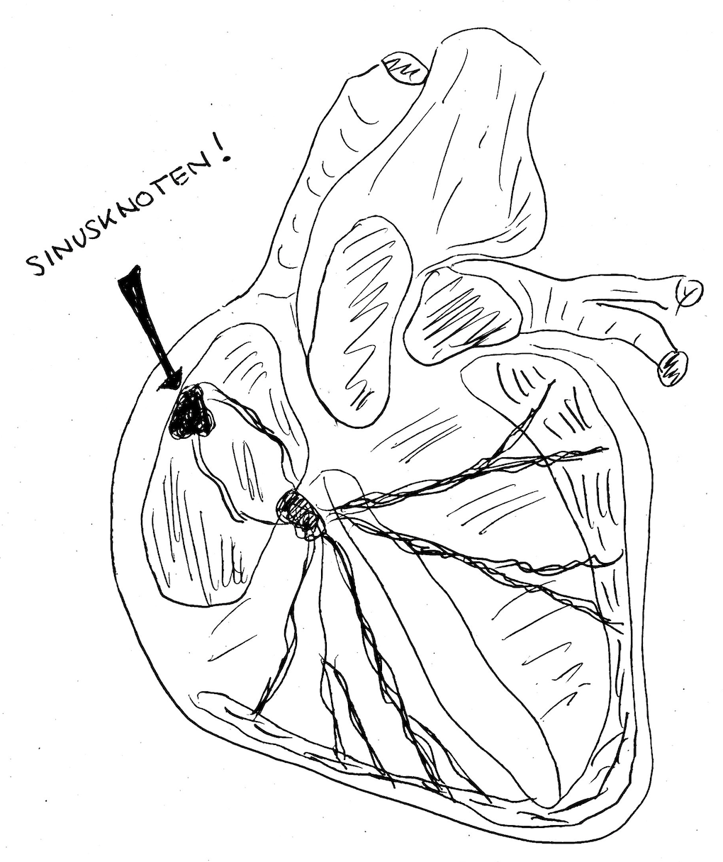
Nerve cells are an example of pulse-coupled oscillators. When the emit action potentials to other neurons, the receiving neuros change their membrane potential and their internal phase that determines when they emit a spike themselves. By this process neuros can attain a synchronous state.
The millenium bridge
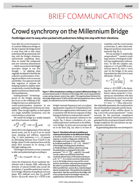
The millennium bridge in London is a suspension bridge that opened operation in June 2000.
Once it was opened, many pededrians crossed it and the bridge began to wobble (lateral movement) due to resonance with the walking rhythms of the pedestrians.
The millennium bridge phenomenon analyzed
In this paper a simple model of phase coupled oscillators describes the conditions for the phenomenon observed during the Millennium Bridge incident.
The state of the bridge is captured by variable $X(t)$ governed by a damped harmonic oscillator, driven by many self-driven oscillators $\Theta_i(t)$ that capture the pedestrians.
$$ M\ddot X + B\dot X +KX=G\sum _i^N\sin(\Theta_i) $$ $$ \dot \Theta = \Omega_i + A\sin(\alpha-\Omega_i) $$
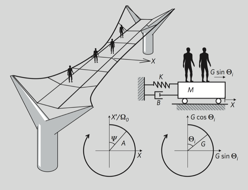
-
Synchronization threshold
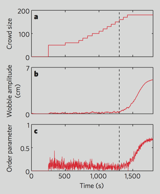
The key finding of the paper was that the spontaneous synchronization of the pedestrians in their gate, and therefore the wobble movement of the bridge depends on the number of people that are on the bridge.
As the number of pedestrians is increased nothing much happens until a certain critical threshold is reached beyond which synchronization sets in.
So, as we change a parameter (number of pedestrians) gradually, the response of the system (degree of synchronizatiom) is not gradual, but abrupt. This is a generic behavior of a critical phenomenon, which we will discuss later in more detail.
-
Types of coupled oscillators
Sometimes we have systems that exhibit spontaneous synchronition in which we have very many interacting oscillators with similar properties
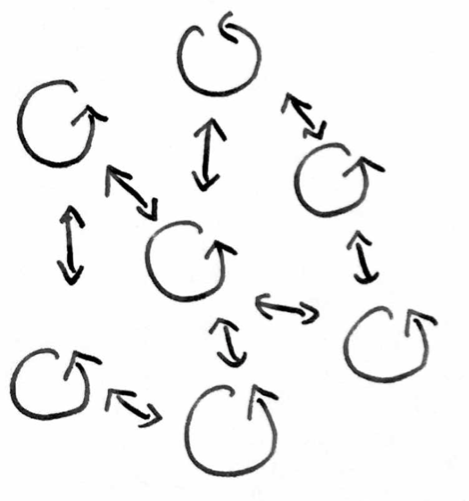
Examples are the fireflies we discussed, or people applauding in synchrony after a concert.
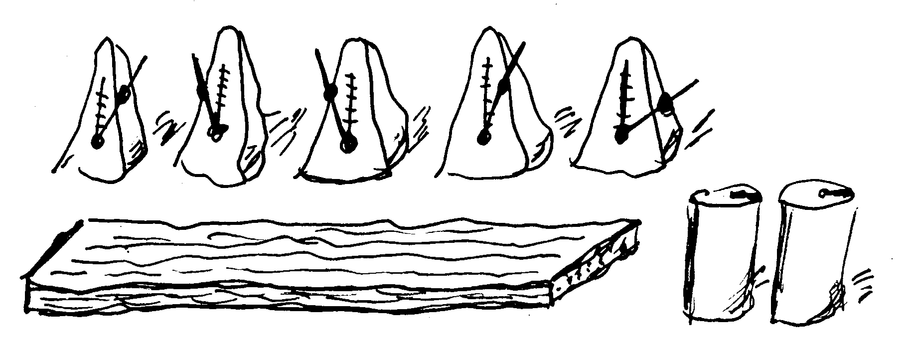
Then there are systems in which a lot of small oscillators are coupled to a larger oscillator that mediates the coupling and synchronization.
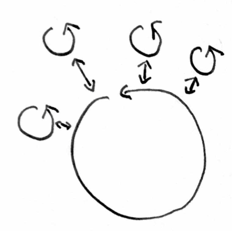
The millennium bridge is such a system, or the metronomes attached to a beam on two empty soda cans.
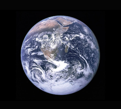
Note: One may be tempted to categorize some systems into this class that really don’t belong in it. Those systems in which an oscillatory, larger system entrains smaller systems and “dictates” their rhythms, e.g. the earths rotation and the circadian rhythm of organisms. In those systems the larger system doesn’t mediate the interaction with the smaller elements.
Steve Strogatz
The Science of Sync
A Good Read
-
Steve Strogatz
Sync
How order emerges from chaos in the universe, nature and daily life.
-
Modeling Synchronization
Phase Coupled Oscillators
Oscillators as dynamic elements
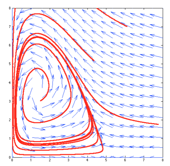
The majority of synchronization phenomena involve oscillators, so systems that can be captured by a periodic state called the phase and typically denoted by $\theta(t)$ which is a periodic variable in the interval $[0,2\pi]$. Sometimes the oscillator is effectively the asymptotic limit-cycle state of an underlying higher dimensional system, like two dimensinal activator-inhibitor system.
The oscillator has a period $T$ and being an oscillator means that $$ \theta(t)=\theta(t+T) $$
The phase velocity is often called the frequency $$ \omega(t)=\dot\theta(t) $$
- -
-
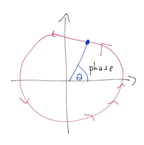
The simplest oscillator
has a constant frequency. It’s best visualized in the $x$-$y$-plane as a dot the moves around in a circle at constant speed.
$\dot{\theta} = \omega $
The Kuramoto Model
The simplest model for phase coupled oscillators
The Kuramoto Model
Phase Coupled Oscillators
We have $N$ oscillators, labeled by $n=1,…,N$ each with its own constant natural frequency $\omega_n$:
$$ \dot{\theta}_n=\omega_n $$
so that
$$ \theta(t) = \theta_0+\omega_n t \quad\text{mod}\quad 2\pi $$
Now we assume that the rate of change of the phase of oscillator $n$ changes as a function of all the other phases, so that in general
$$ \dot{\theta}_n=\omega_n + f_n(\theta_1,…,\theta_N) $$
Note: Each oscillator can have it’s own function $f_n$.
Two Oscillators
Let’s first just consider two oscillator
$$ \dot{\theta}_1=\omega_1 + f_1(\theta_1,\theta_2) $$
$$ \dot{\theta}_2=\omega_2 + f_2(\theta_1,\theta_2) $$
Each oscillator moves forward with its own natural frequency $\omega_i$. The force of oscillator $2$ exerted on $1$ is defined by the function $f_1$, the force of oscillator $1$ exerted on $2$ is defined by function $f_2$. In general these $f_1\neq f_2$ functions can be different
Assumption 1
We simplify a bit and assume that the interactions are symmetric which means that the equations
$$ \dot{\theta}_1=\omega_1 + f_1(\theta_1,\theta_2) $$
$$ \dot{\theta}_2=\omega_2 + f_2(\theta_1,\theta_2) $$
become
$$ \dot{\theta}_1=\omega_1 + f(\theta_1,\theta_2) $$
$$ \dot{\theta}_2=\omega_2 + f(\theta_2,\theta_1) $$
So there’s now only one interaction function $f$ instead of two. Note also that because of the symmetry the arguments are reversed in the second dynamic equation.
Assumption 2
Now we assume that the interaction only depends on the phase difference so
$$ \dot{\theta}_1=\omega_1 + f(\theta_1,\theta_2) $$
$$ \dot{\theta}_2=\omega_2 + f(\theta_2,\theta_1) $$
turns into
$$ \dot{\theta}_1=\omega_1 + f(\theta_2-\theta_1) $$
$$ \dot{\theta}_2=\omega_2 + f(\theta_1-\theta_2) $$
This means that the absolute phase positions do not matter. If I rotate the entire system by some angle, nothing changes. Or alternatively if I tilt my head and look at the system nothing changes.
fixing the function $f$
-
Now just consider the term $f(\theta_2-\theta_1)$ in
$$ \dot{\theta}_1=\omega_1 + f(\theta_2-\theta_1) $$
$$ \dot{\theta}_2=\omega_2 + f(\theta_1-\theta_2) $$
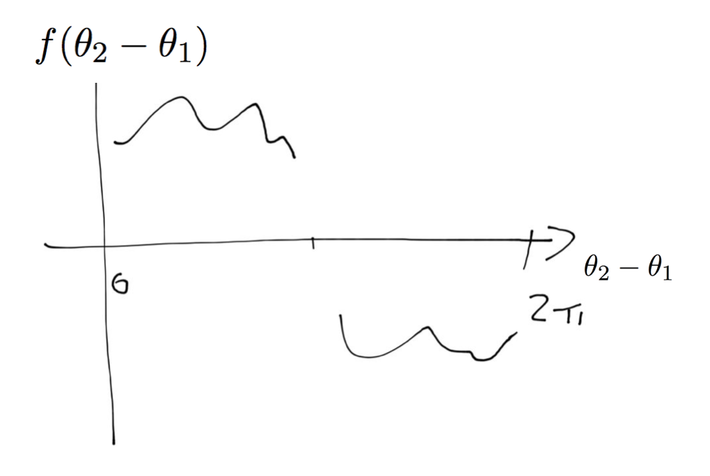
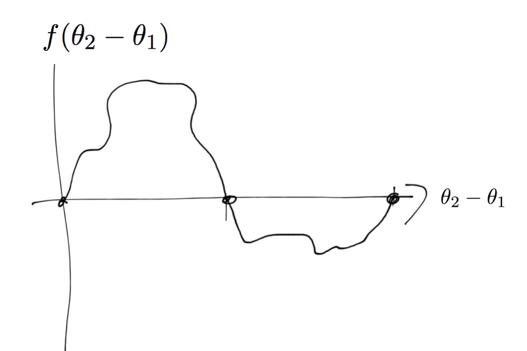
Let’s say that $(\theta_2-\theta_1)\; \text{mod} \; 2\pi < \pi$ which means that oscillator 2 is ahead of oscillator 1. By “ahead” on a circle we mean, that oscillator 1 has a shorter angular distance to move to catch up to oscillator 2 that vice versa. In this case we would like oscillator 1 to “catch up” by increasing it’s speed so we want $f(\theta_2-\theta_1)>0$ which implies that 1 is moving a bit faster. Likewise, oscillator 2 is slowing down. If on the other hand oscillator 2 is trailing 1, we have $$ 2\pi > (\theta_2-\theta_1) \;\text{mod}\; 2\pi > \pi $$ and in this case we would like 1 to slow down and 2 to accelarate so in this case we want $f(\theta_2-\theta_1)<0$.
-
So the function $f(\theta_2-\theta_1)$ should look like this
Finally…
-
we require a continuous function….
-
The simplest coupling function is therefore a simple sine:
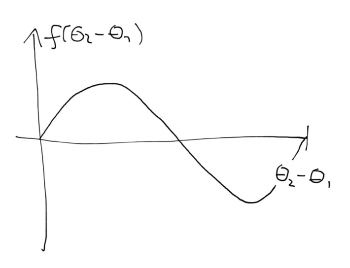 so
so$$ f(\theta_2-\theta_1)=\frac{K}{2}\sin(\theta_2-\theta_1) $$
where the parameter $K$ is proportional to the amplitude of the sine.
The Kuramoto Model for two oscillators
with this we arrive at:
$$ \dot{\theta}_1=\omega_1 + \frac{K}{2}\sin(\theta_2-\theta_1) $$
$$ \dot{\theta}_2=\omega_2 + \frac{K}{2}\sin(\theta_1-\theta_2) $$
which is the Kuramoto Model for two oscillators. The parameters are the two natural frequencies $\omega_1$ and $\omega_2$ as well as the coupling constant $K$.
Analysis
given the two oscillator Kuramoto model:
$$ \dot{\theta}_1=\omega_1 + \frac{K}{2}\sin(\theta_2-\theta_1) $$
$$ \dot{\theta}_2=\omega_2 + \frac{K}{2}\sin(\theta_1-\theta_2) $$
we first let $x=\theta_2-\theta_1$ and the two equations simplify to a single variable dynamical system
$$ \dot{x}=\delta\omega - K \sin(x) $$
wher $\delta\omega=\omega_2-\omega_1$ is the different in natural frequencies.
Analysis
we can now analyse this with the graphical techniques for one-dimensional dynamical systems. We just draw the function
$$ f(x)=\delta\omega-K\sin(x) $$
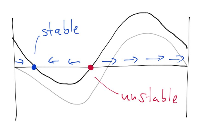
and we see that if
$$ K > K_c = \delta\omega $$
the system has two fixpoints, a stable one and an unstable one. The stable fixpoint is given by the smaller solution to
$$ x^\star=\theta_2^\star-\theta_1^\star=\alpha=\sin^{-1}(\delta\omega/K). $$
If on the other hand
$$ K < K_c = \delta\omega $$
we have $f(x)>0$ on the entire range $[0,2\pi]$ which means no fixpoints exist, and $x(t)=\theta_2(t)-\theta_2(t)$ is always increasing (mod $2\pi$).
Also, if both oscillators have the same natural frequency $\omega_1=\omega_2$ and $\delta\omega=0$, for arbitrarily small coupling strength $K$ the two oscillators will synchronize.
Summary
This implies that:
- if both oscillators have identical natural frequencies $\delta\omega=0$, they always synchronize with zero phase difference $\alpha=0$.
- if the natural frequencies differ the oscillators snychronize only for a coupling that is larger than a critical value $K_c=\delta\omega$.
- if they synchronize they have a phase difference $\alpha=\sin^{-1}(\delta\omega/K)$.
- in the asymptotically stable state the rate of change of both oscillators is the same and identical to the mean of their natural frequency.
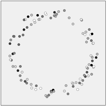
More than two oscillators
The Kuramoto Model is easily generalized to $N$ oscillators as in this picture.
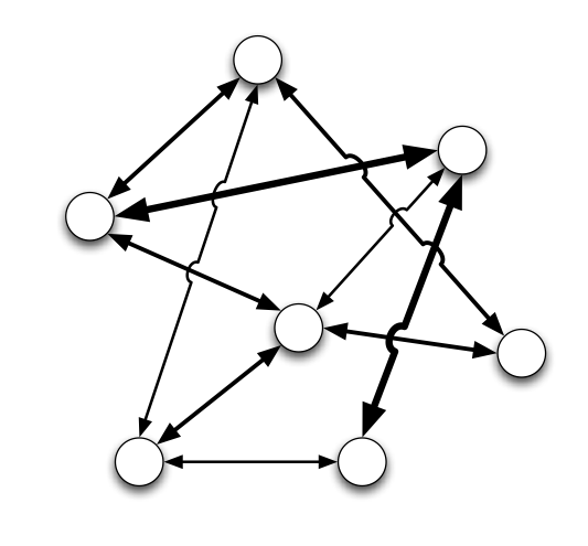
$$ \dot{\theta}_n=\omega_n + \frac{1}{N}\sum _m K _{nm}\sin(\theta_m-\theta_n) $$
In this case the coupling of the different oscillators is defined by a coupling matrix $K_{nm}$ that is typically symmetric. In general this system is difficult to analyse systematically and depending on the coupling matrix lots of different things can happen.
Explore the Kuramoto model
You can explore the Kuramoto model with these complexity explorables
Click on images to go to the explorables.
Critical Phenomena

Remember Kuramoto
$$ \dot x = \delta\omega-K\sin(x) $$
SIS Model
$$ \dot x = \alpha x (1-x)-\beta x $$ $$ R=\alpha/\beta $$
$$ R<1 $$ $x^\star=0$ is a stable fixpoint
$$ R>1 $$ $x^\star=0$ is unstable
$x^\star=1-1/R$ is a stable fixpint
Weird SIS Model
$$ \dot x = \alpha x^2 (1-x)-\beta x $$
Saddle node bifurcations everywhere
$$ \dot x = \sin(3x)+x^2/5+\mu $$
Tipping points
$$ \dot x = -x(x-1)(x+1)+\mu $$ $$ \dot x = -x^3+x+\mu $$
Hysteresis
$$ \dot x = -x(x-1)(x+1)+\mu+\text{Noise} $$
Branching
$$ \dot x = \mu x - x^3 $$
Pitchfork Bifurcation
$$ \dot x = \mu x - x^3 $$
Critical Phenomena in Space
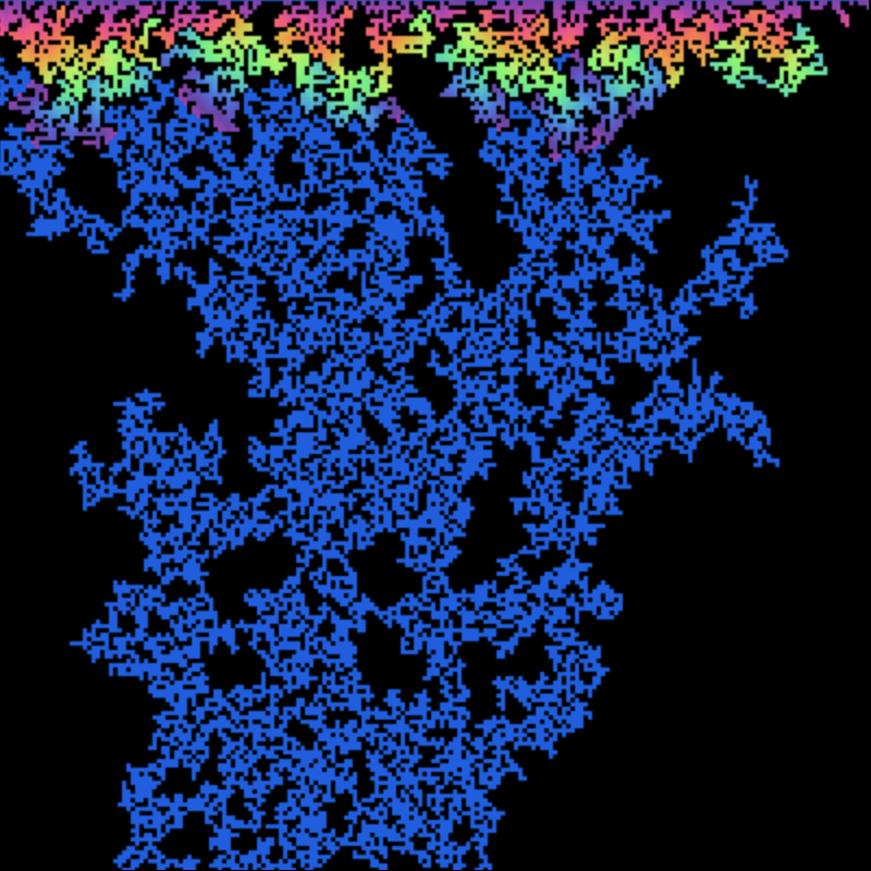
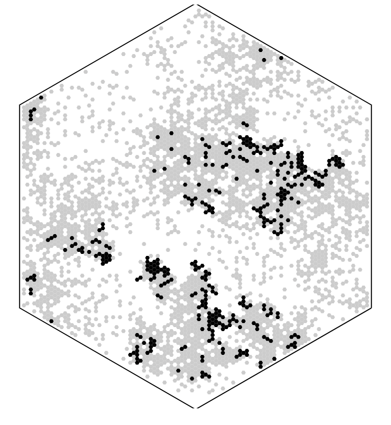
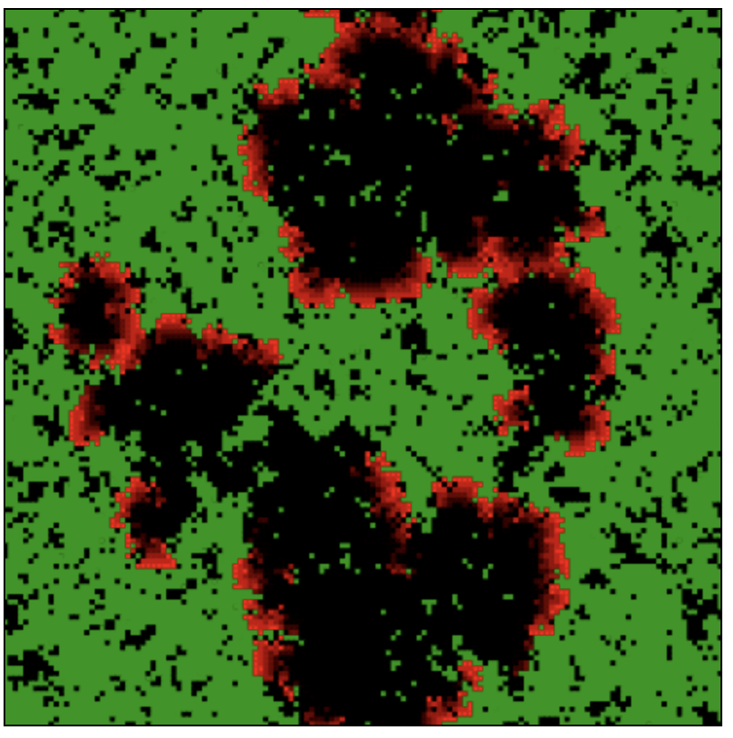
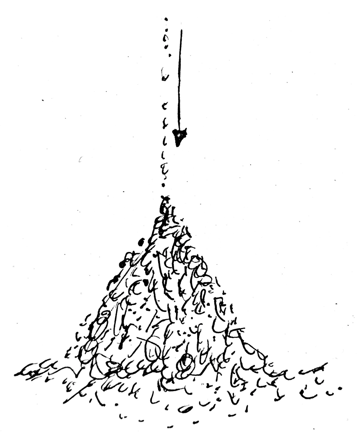
Self-Organized Criticality
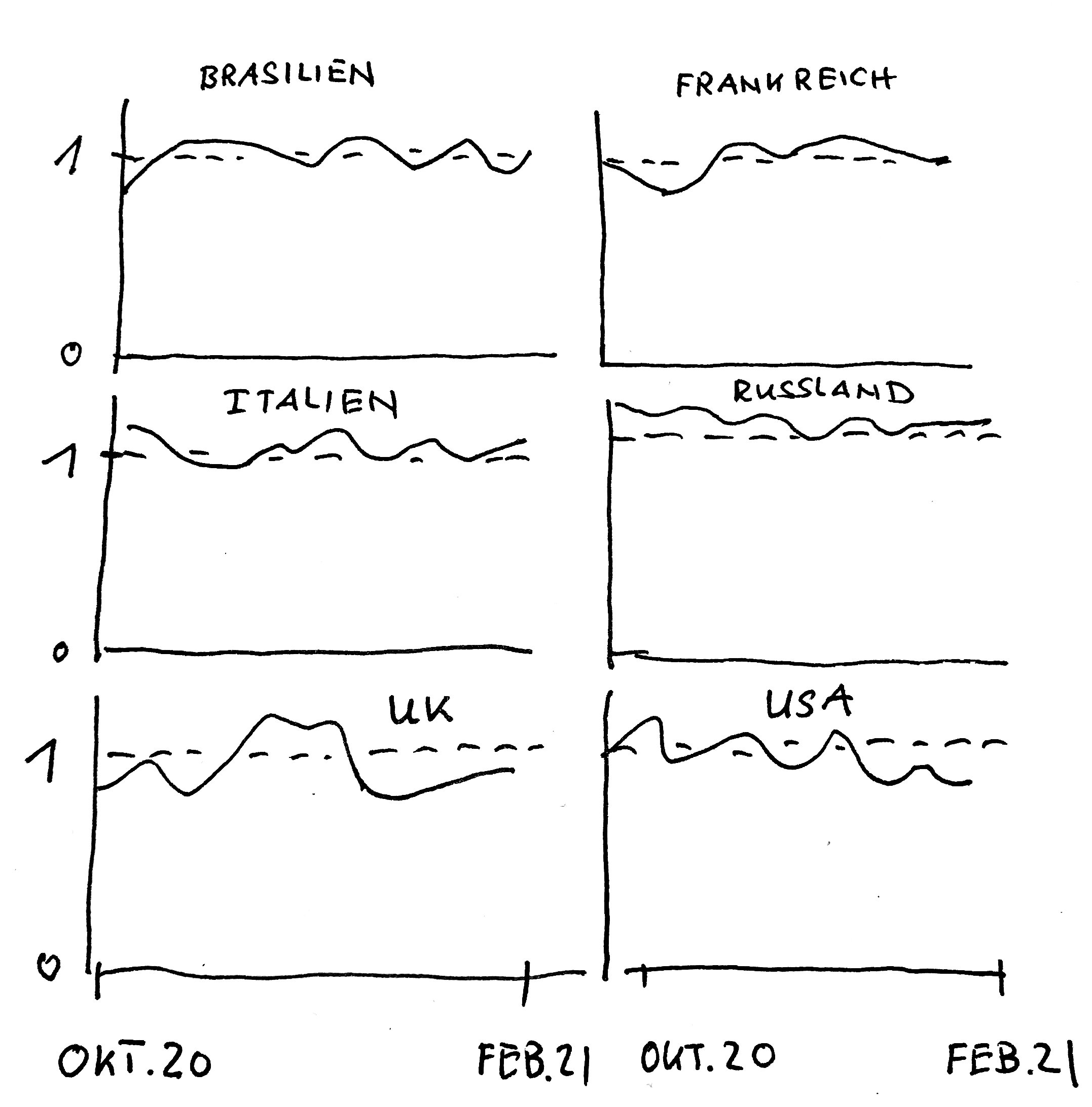
Self-Organized Critical Covid Pandemic
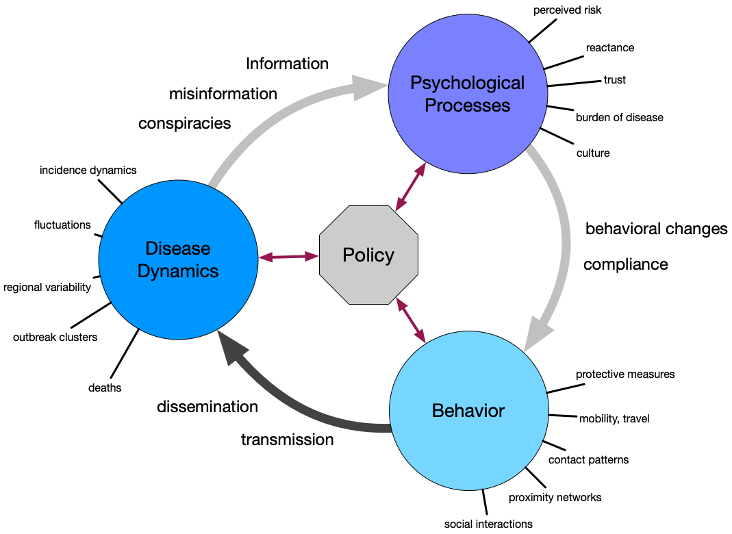
Self-Organized Critical Covid Pandemic
-
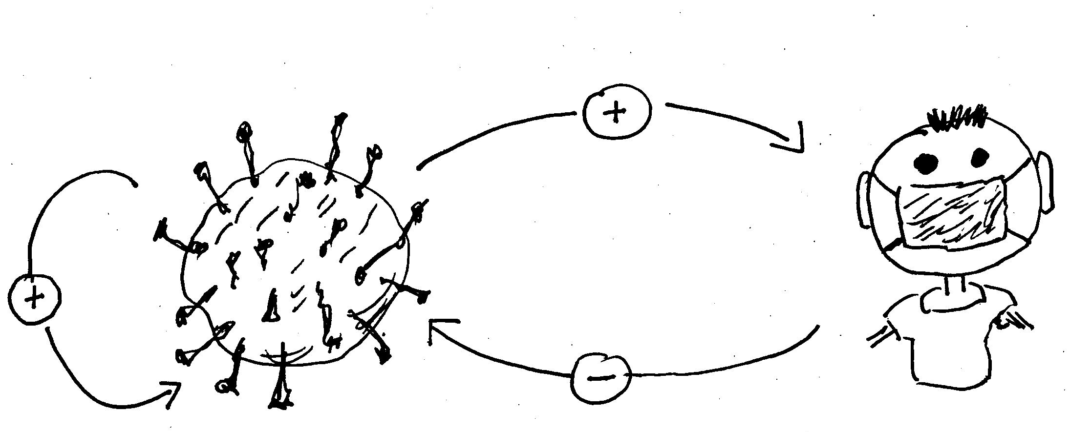
Basic Reproduction value R
Pattern Formation
From a homogeneous state to structure
Examples: Ripples in the sand
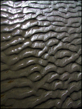
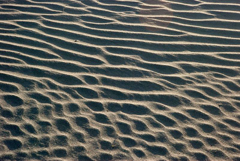
These stripes and patches form by an amplification of small perturbations by laminar wind / water flow across the surface.
Morning Glory
Morning Glory is a cloud phenomenon that exhibits long regular rotating rolls with regular spacing. They are a rare meteorological phenomenon.
fractal, self-similar patterns
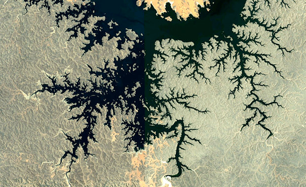
This sattelite image of a river system exhibits fractal / self-similar geometry.
Rayleigh–Bénard Convection
When a thin film of oil in a pan is heated from below the heat gradient is too large for heat dispersion to distribute the heat. As a result convection cells emerge that transport heat from the bottom to the surface.
Belousov–Zhabotinsky reaction
The BZ reaction is an activator-inhibitor systems that exhibits oscillatory behavior in a well mixed container.
Belousov–Zhabotinsky reaction
The BZ reaction in a thin film on a petri-dish exhibits characteristic target patterns and spiral waves. It’s one of the most famous systems known to exhibit this behavior.
Dictyostelium discoideum
The organism Dictyostelium discoideum is an amoeba, a slime mold that exhibits interesing behavior. In one mode it has a single cell life-style. When food runs out the cells signal to their environment and aggregate, form a multi-cellular organism and cells differentiate.
Dictyostelium discoideum and cAMP
This video shows the dynamics of the signaling molecule cAMP that Dictyostelium discoideum uses to aggregate. When individuals are exposed to cAMP the move up the cAMP gradient and excrete cAMP themselves.
Pattern formation in the brain
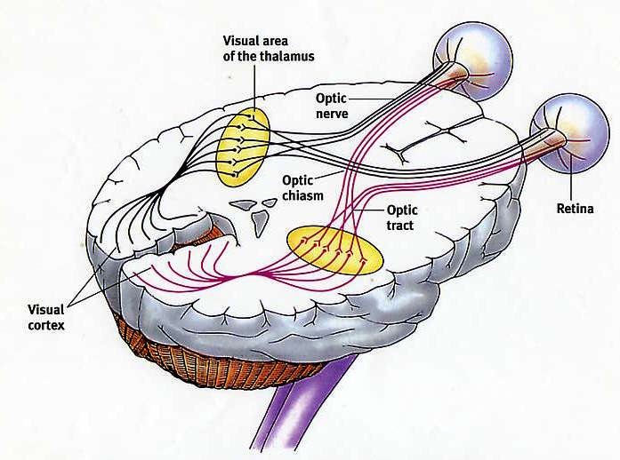
Optical pathways in the brain: Each eye splits the visual field into left/right hemispheres. The axonal fibers from each of the two eyes and two hemispheres get distributed to the left/right visual cortices in the back of the brain, such that the left visual cortex receives information from the left visual field (from both eyes) and the right visual cortex from the right visual field.
Ocular Dominance Maps
Cells in the visual cortex exhibit an ocular dominance. They exhibit the tendency to respond to stimuli presented to one eye more than those presented to the other eye. As a function of location on the visual cortex the ocular dominance patterns consists of stripes of a specific wave-length.
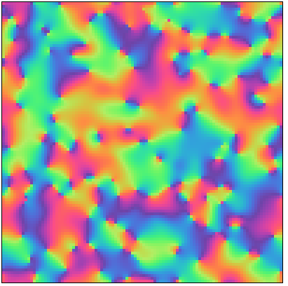
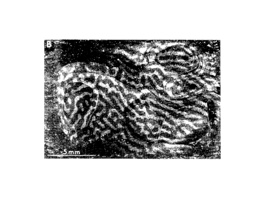
Orientation maps in the visual cortex
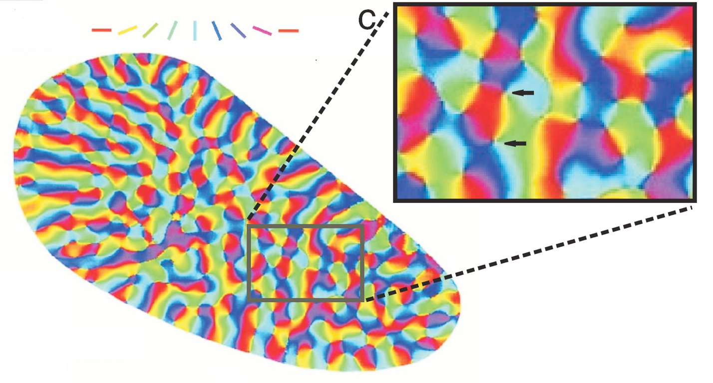
Some cells in the visual cortex exhibit an orientation preference, they respond primarily to visual stimuli on the retina that are oriented in a specific direction. When the entire visual cortex is mapped and the orientation preference mapped in color for many species we see an orientation map. This map exhibits characteristic pinwheels, singularities in the orientation preference.
Patterns on Snails and Shells
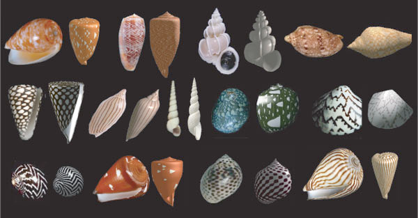
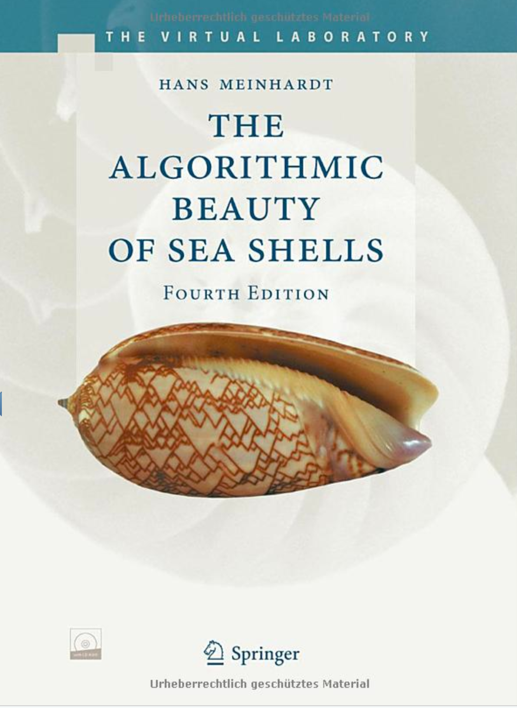
Some species of snails and sea shells exhibit complex patterns on their surface. How these emerge and can be classified is discussed in a grear book by Hans Meinhardt: The Algorithmic Beauty of Sea Shells.
Animal Coats
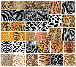
One of the most prominant examples of pattern formation in biology are patterns on animal coats. Typically they come in stripes or semi-regular patches.
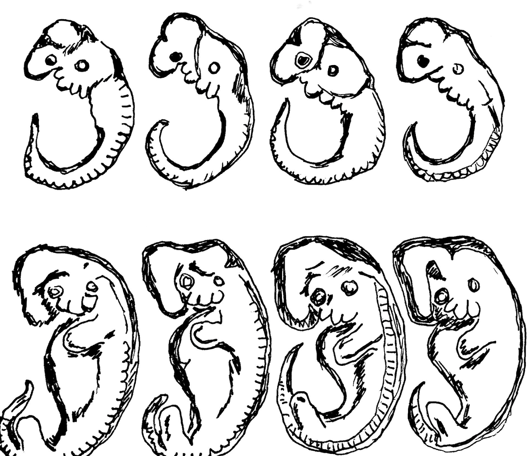
Embryogenesis
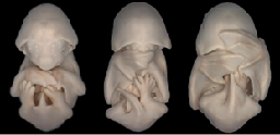
The most sophisticated phenomenon of pattern formation is embryogenesis which can be understood as a sequence of pattern forming events that gain more and more complexity. The image depicts the embryo of a bat.
Morphogenesis and Gene Regulation
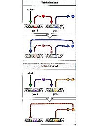
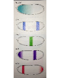
The way this is accomplished? In morphogenesis genes that are play a role in the process regulate each other and eventually are expressed in a spatially inhomogeneous pattern. For example in the embryo of the fruitfly different genes are expressed in stripes across the embryo which eventually leads to the segmentation of the embryo.
Morphogenesis in the Fruitfly Embryo
This video shows the development of a fruitfly embryo in toto.
Digits and the Turing Mechanism
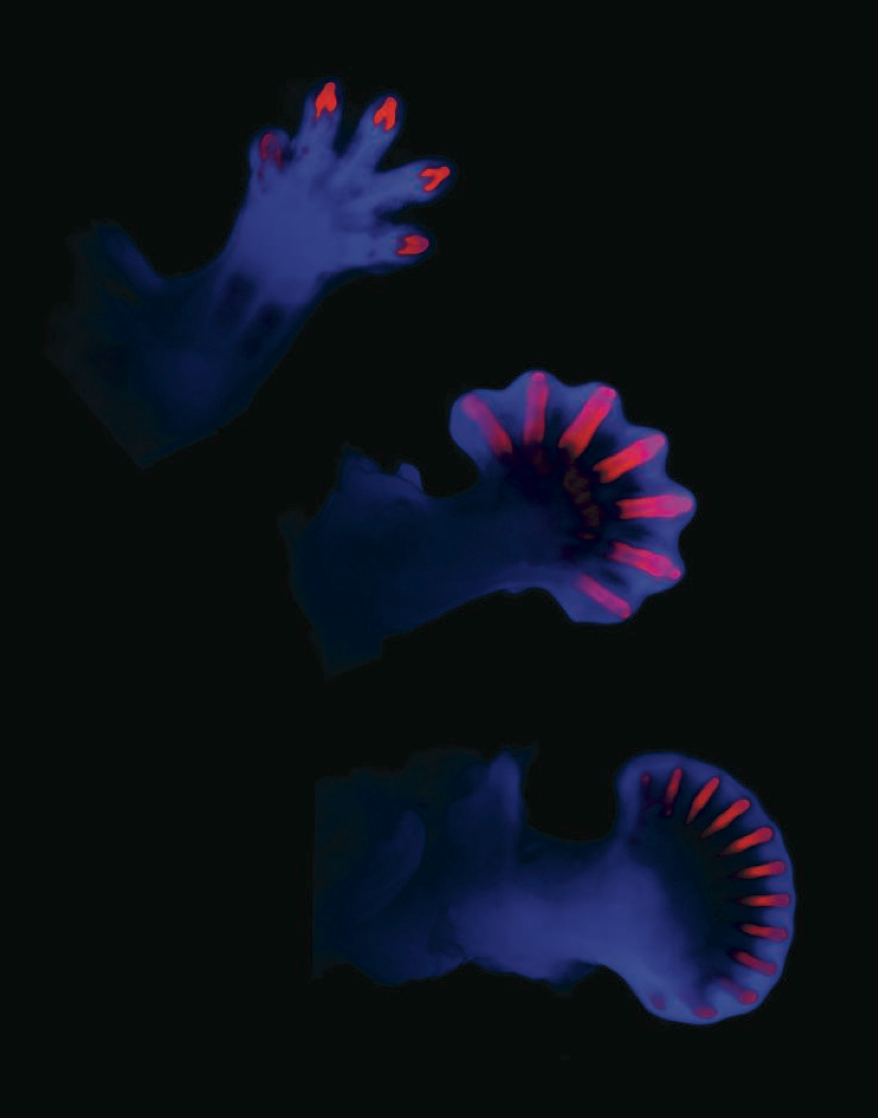
This image was taken from the paper Hox Genes Regulate Digit Patterning by Controlling the Wavelength of a Turing-Type Mechanism that shows that the digit development is driven by the Turing Mechanism, one of the key mechanisms in which patterns self-organize from a homogeneous states.
Patterns in Collective Behavior
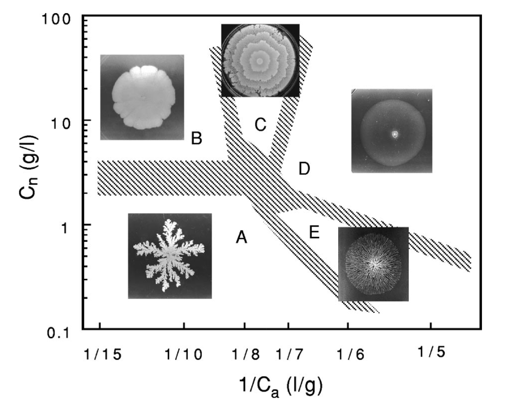
Patterns also appear in collective behavior in colonies of microbes.
Alan Turing & the Turing Mechanism
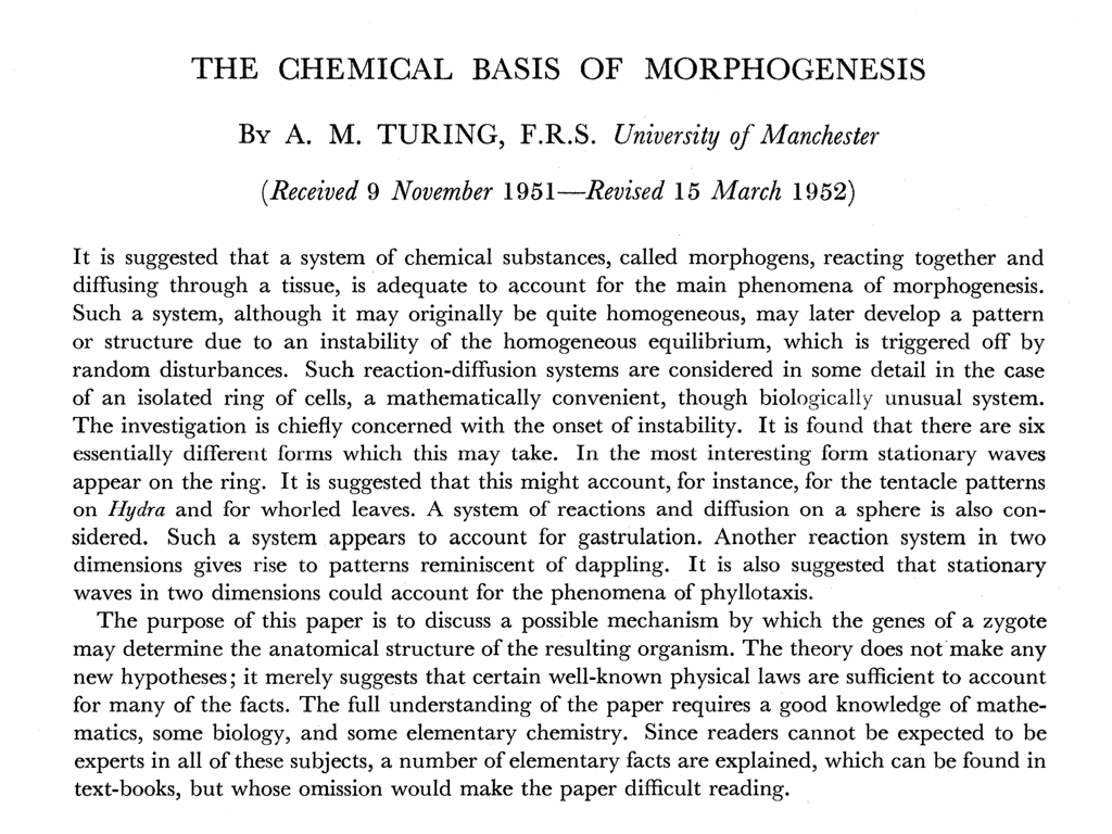
An important mechanism that we will discuss in class was discovered by Alan Turing and published in the above paper. It’s a seminal paper on the topic and was very important for understanding how patterns may emerge in biological systems.
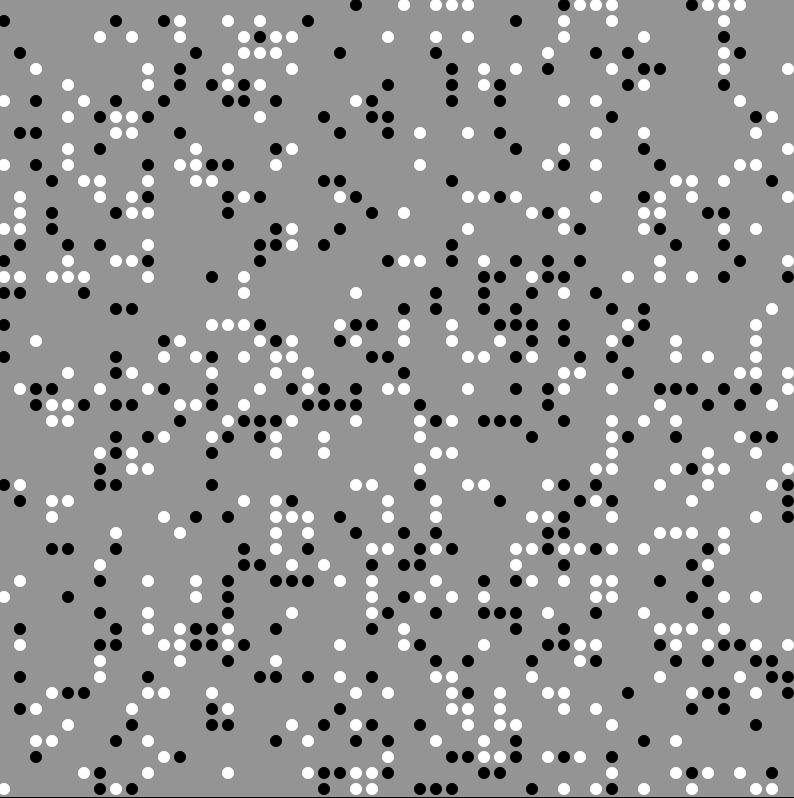
First steps in Modelling: Voter Model
The original voter model is a discrete time model on a square lattice. Each lattice point has a binary state, it can either be $1$ or $-1$ for example.
$$ u_{nm} = 1\qquad\text{or}\qquad u_{nm} = -1 $$
These are the rules for the voter model
- The system (square lattice) is initialized in some configuration, e.g. with probability $1/2$ a lattice site is set to $1$ with probability $1/2$ set to $-1$.
- Pick a random lattice site $n$
- Pick one of its 8 neighbors at random (labeled $m$)
- Site $n$ adopts the state of neighbor $m$
- Go back to step 1
The Majority Model
This is similar to the Voter Model. But instead of adopting the “opinion” of a randomly chosen neighbor, a site adopts the majority opinion of the neighbors. When no majority is there, the site picks a random state (either $1$ or $-1$)
These are the rules for the voter model
- The system (square lattice) is initialized in some configuation, e.g. with probability $1/2$ a lattice site is set to $1$ with probability $1/2$ set to $-1$.
- Pick a random lattice site $n$
- Compute the majority opinion of the neighborbood
- Site $n$ adopts the state of the majority if it exists, when opinions are tied, the site picks the opinion of a randomly chose neighbor
- Go back to step 1
Voter and Majority Model
Classically only two states are possible for each lattice site. Both voter and majority model are easily generalized to more than two opinions (states).