The SIR-X model is described in detail here: Effective containment explains sub-exponential growth in confirmed cases of recent COVID-19 outbreak in China, B. F. Maier & D. Brockmann, Science, eabb4557, DOI: 10.1126/science.abb4557, (2020)
The model
Traditional epidemiological models for the spread of infectious diseses do not take into account population-wide behavior changes that directly impact outbreak dynamics. Because of the containment strategies implemented worldwide in response to the COVID-19 pandemic, these models are unsuited to accurately track the number of infected individuals.
Therefore, we present a novel model in which the transmission rate changes over time, inspired by the assumption that susceptible individuals are continuously removed from the transmission process due to interventions such as social distancing, public shutdowns, quarantines, and curfews.
Classic SIR dynamics
In order to reflect the dynamics of an outbreak, simple epidemiological models divide the general population into several compartments. In the SIR model, people are categorized as (S)usceptible to infection, (I)nfected and infectious, or (R)emoved from the process due to recovery, immunity, quanantine or death.
Infectious diseases are transmitted by contacts between susceptible and infectious individuals. Compartmental models assume a well-mixed population in which the number of possible transmissions at any given time is proportional to the total number of possible infectious contacts \( S \times I \) where \( S \) represents the fraction of people susceptible in the population and \( I \) is the fraction of infected people.
This means that the number of susceptible individuals declines over time, following the ordinary differential equation (ODE)
[ \frac{dS}{dt} = -\alpha SI. ]
Here, \( \alpha \) is the reproduction rate of the process which quantifies how many of the potential susceptible-infectious contacts lead to new infections per day.
Consequently, the number of infected individuals increases by the same amount. At the same time, infected individuals can also recover or be removed from the population. This is reflected by the ODEs
[ \frac{dI}{dt} = \alpha SI - \beta I ] [ \frac{dR}{dt} = \beta I, ]
with \( \beta \) quantifying the number of infected people that cease to take part in the transmission process per day.
In the initial stages of an outbreak when the number of infected individuals is relatively low and most people fall into the susceptible compartment, one can safely assume that \( S \approx 1\) . Following this assumption, the differential equation for the fraction of infected individuals \( \frac{dI}{dt} \) becomes linear and is satisfied with a funciton of exponential growth, such that
[ I(t) \approx I_0 \exp\{(\alpha-\beta)t\} . ]
This exponential increase of infections is observed under unconstrained conditions. In the COVID-19 outbreak, we can also see this pattern of growth in countries where containment measures were implemented at a relatively late stage in the outbreak, such as in the United States.
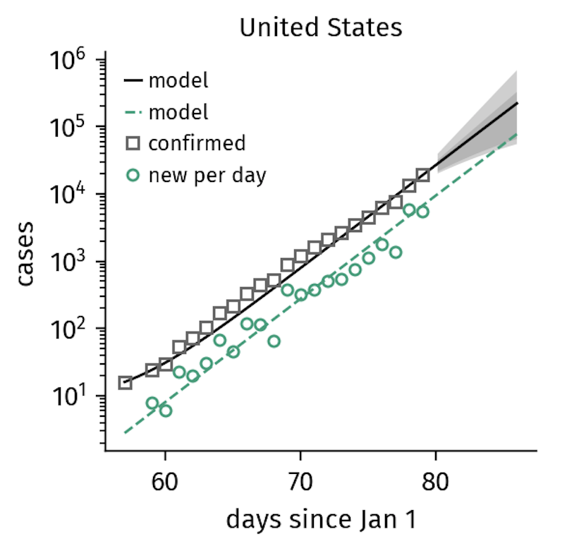
Figure 1. The number of confirmed cases in the US continues to grow exponentially, reflecting the lack of interventions other than quarantine. Note that it takes several days for policy changes to be reflected in the data, which is why the US growth numbers might follow a slower trajectory soon (as of March 21). The model curves shown here represent the SIR-X-model that will be introduced in the next section.
However, in countries such as Italy, the implementation of increasingly stricter containment interventions altered the spreading dynamics resulting in a sub-exponential pattern of growth.
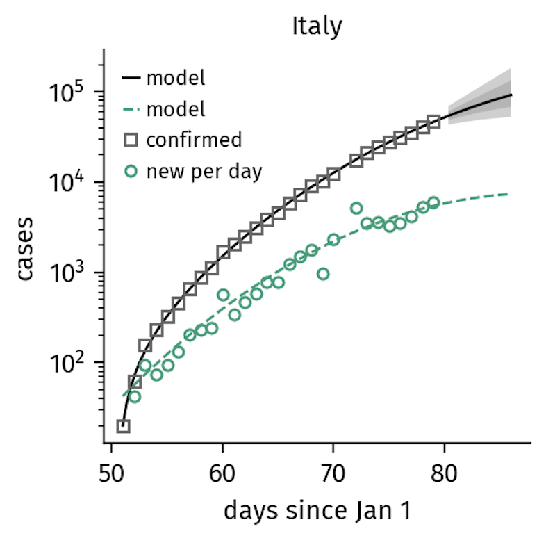
Figure 2. Italy
implemented gradually increasing containment measures that explain the
sub-exponential growth in confirmed cases now seen (as of March 21).
Here, the containment rate
is of similar order as the time scales of the unfolding disease.
SIR-X dynamics: Outbreaks with temporally increasing interventions
In case of a severe outbreak such as the COVID-19 epidemic, the public can counteract growth by changing the structure of contact behavior, such that the number of potential transmissions is reduced. There are several means of achieving this:
Quarantine: Symptomatic individuals are isolated. This removes infected people from the \( I \) compartment at a quarantine rate \( \kappa \).
Contact tracing: Contacts of identified infected are traced and put under isolation for the maximal incubation time. This is a very effective strategy if implemented early enough, as demonstrated by countries like Singapore and Taiwan. Almost the entire pool of susceptible individuals are removed from the transmission process before they have a chance to become infected, much like a firebreak shields large parts of a forest during forest fires.
Social distancing: The number of potential contacts decreases as physical distance between people increases. This containment effort often occurs in response to a growing outbreak with a large number of unknown infections. Specific measures include self-isolation, cancellation of events, and increased hygienic measures such as hand washing.
Public shutdown: The closure of public institutions including schools and non-essential businesses decreases potentially infectious contacts.
Lockdown: Mandatory curfews and travel restrictions decrease mixing in the population and, consequently, infectious contacts.
The severity of containment measures progresses gradually as an outbreak unfolds and more drastic interventions are deemed necessary. Given this, it is reasonable to assume a gradual depletion of susceptible individuals that are shielded from infection.
In order to account for this continuous change in contacts, we introduce a general containment rate \( \kappa_0 \) at which susceptibles are removed from the transmission process.
Additionally, we assume that infected individuals are quarantined at a quarantine rate \( \kappa \). Because containment measures affect people who are unknowingly infected in addition to the pool of healthy susceptible people, both \( \kappa_0 \) and \( \kappa \) have an effect on the fraction of infected individuals as well.
The complete model is given by the equations
[ \frac{dS}{dt} = - \alpha SI - \kappa_0 S ] [ \frac{dI}{dt} = \alpha SI - \beta I - \kappa_0 I - \kappa I ] [ \frac{dX}{dt} = (\kappa_0 + \kappa) I ] [ \frac{dR}{dt} = \kappa_0 S + \beta I, ]
where \( X \) is the number of quarantined individuals. Essentially, the exponential depletion of the number of people susceptible to the transmission process yields sub-exponential growth in the quarantined population. We assume there is a constant average duration between when an infected is tested and the date their result is announced.
How we do forecasts
The equations above can be integrated numerically, but no closed-form solutions exist. We perform simple Levenberg-Marquardt fits, minimizing the mean squared distance between the data (confirmed cases \( C(t) \) ) and the obtained numerical prediction \( X(t) \) to find the initial number of unidentified infected persons \( I_0 \), the containment rate \( \kappa_0 \) and the quarantine rate \( \kappa \).
For all countries, we assume a fixed basic reproduction number of \( R_0 = \alpha/\beta = 3.07 \) and a removal rate of \( \beta = 0.38\mathrm{d}^{-1} \) (mean infectious time of \( T_I = 1/\beta = 2.6\mathrm{d}\) ). These values are consistent with reported estimates and fits well with the case number developments in all countries to date. An infectious period of \( T_I = 2.6\mathrm{d}\) corresponds to roughly only one third of the reported average infectious period of moderate cases in Mailand China.
How well does this model predict the future?
Predicting case numbers in epidemics is a bit like predicting the weather. Within a single day, there are factors that can affect how the number of infected people will change, including systematic errors like delay in testing, logistic restriction in testing, failure of reporting infrastructure, abruptly introduced changes to transmission dynamics, or just due to noise.
Nevertheless, the median success of this model’s predictions remains stable for at least 5 days. We quantify this by computing the over-/underestimation factor of
[ f = \frac {\mathrm{prediction}} {\mathrm{true\ value}} ]
and evaluating the accuracy of model prediction for 1-6 days in the future, beginning for fits on March 13 until March 19. The median prediction factor is virtually \( f = 1.0 \) for 5 days, decreasing to \( f = 0.86 \) for the 6th day. We therefore present predictions for 6 days only.
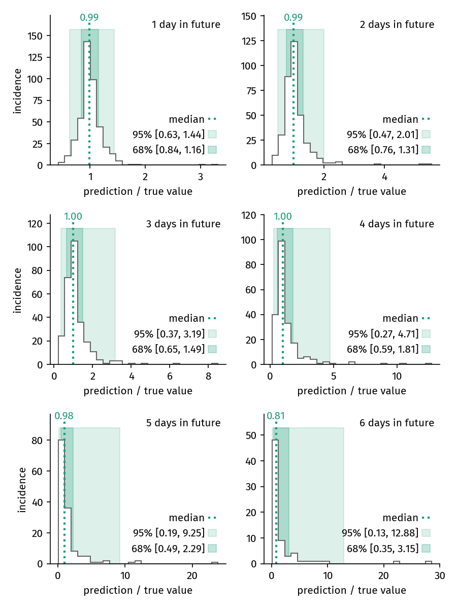
Figure 3. Distribution of prediction factors for predictions of 1 to 6 days. For predictions until up to 5 days, the median prediction factor is virtually \( f = 1 \). The variance of the prediction success increases with each subsequent day in the future.
This figure shows how the distribution of predictions changes when looking increasingy further into the future. The variance of the prediction factor continuously increases with time.
Our model is intentionally sensitive to trends developing within the last days in order to reflect the latest developments well. As a consequence, a sudden and drastic change in the reported new infections might potentially trigger under- or overestimation of case numbers in the following days. We therefore apply the following procedure to estimate prediction uncertainties.
Let \( (t_f, C(t_f) )\) be the most recent data point of a time series. We first estimate the case number for the next day \( C(t_f+1\mathrm{d}) \) by fitting the model to the time series and setting \( C(t_f+1\mathrm{d}) = X(t_f+1\mathrm{d})\). Then, we add \( (t_f+1\mathrm{d}, f_b X(t_f+1\mathrm{d})\) as a new data point, where \( f_b \) is equal to one of the four bounds of the 95% and 68% confidence intervals for the prediction factor’s distribution of 1 day into the future. For each of the four new virtual time series, we refit the model to see what it would predict had we drastically under- or overestimated the original data point. These curves represent the red and grey shaded regions around the prediction.